Population Ecology, part 1
Principles of Ecology Week 2
Reminder - self reflection due on Sunday
Prompt and submission available on Moodle.
For next week: See “Week 3 Activities” on class website or Moodle (read peer-reviewed paper and listen to a podcast episode) . . .
Reminder - complete weekly readings before class
Today’s lecture covers material from Chapter 1 of Gotelli’s Primer of Ecology (link)
On Friday, we will begin to cover structured population growth, which is introduced in this video
Opportunity for logistical questions
Bird Walk at BREC this Saturday
Population ecology
What defines a population?
Individuals of the same species living together
Individuals interact with one-another
e.g. mating, facilitating, competing
Photo by Jeffrey Hamilton on Unsplash
Photo by National Cancer Institute on Unsplash
How does a population grow or shrink?
- Birth (+)
- Death (-)
- Immigration (individuals coming in, +)
- Emigration (individuals leaving, -)
How does a population grow or shrink?
- Birth (+)
- Death (-)
- Immigration (individuals coming in, +)
- Emigration (individuals leaving, -)
For now, we will consider a ‘closed’ population
How does a population grow or shrink?
In a closed population, population size (\(N\)) only changes due to births and deaths
\[N_{t+1} = N_{t} + B - D\]
\[N_{t+1} - N_{t} = B-D\]
\[\Delta N = B-D\]
\[\frac{dN}{dt} = B-D\]
How does a population grow or shrink?
\[\frac{dN}{dt} = B-D\]
We need to know: What determines \(B\) and \(D\)?
Depends on the birth rate and mortality (death) rate:
- Total births = per-capita birth rate * number of individuals
\[B = bN\]
- Total deaths = per-capita mortality rate * number of individuals
\[D = dN\]
How does a population grow or shrink?
\[\frac{dN}{dt} = B-D\]
\[B = bN \text{ and } D = dN\]
\[\frac{dN}{dt} = bN - dN\]
\[\frac{dN}{dt} = (b- d) N\]
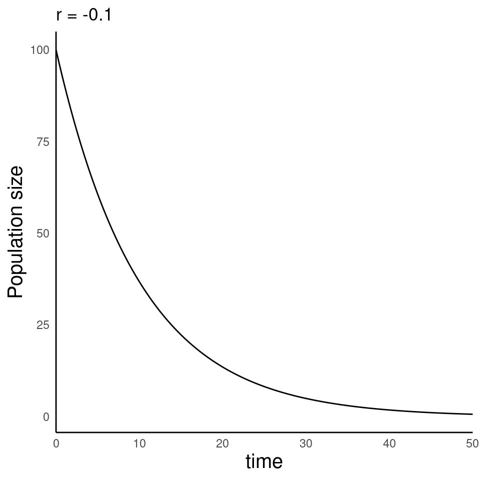
\[\boxed{\frac{dN}{dt} = rN}\]
Populations grow when there are more births than deaths (\((b-d) > 0\); aka \(r > 0\))
Populations shrink when there are more deaths than births (\((b-d) < 0\); aka \(r < 0\))
The magnitude of \(r\) determines the rate of growth
How can such a simple population model help?
Source: Wikimedia
Recall that the magnitude of \(r\) determines the rate of growth
What happens when \(r = 0\)?
Equilibrium in ecology
\(r = 0\), when the rates of birth and death are equal to one another (\(b-d = 0\))
When this is true, the total number of births cancels out the total number of deaths, meaning the population size does not change.
\[\frac{dN}{dt} = rN = 0\]
This is the equilibrium state of the system.
Note that “equilibrium” doesn’t mean “nothing is changing”: there will be new births, and new deaths.
But they cancel each other, and the population size remains constant.
Equilibrium in ecology
\[\frac{dN}{dt} = rN = 0\]
This is the equilibrium state of the system.
The exponential growth model has two equilibrium conditions. One is that \(r = 0\). What is the other?
We will be exploring the equilibrium conditions for many of the models we introduce through the semester, because it has been a central concept in ecology.
How math helps us derive insights from the model
\[\frac{dN}{dt} = rN\]
- If we integrate this model, we can predict population size at any time in the future:
\[N_t = N_0*e^{rt}\]
- We can also predict how long it takes a population to double in size (‘doubling time’):
\[t_{\text{doubling}} = \frac{\text{ln}(2)}{r}\]
The exponential growth model: summary
We can imagine that the dynamics of a population (i.e. how does population size change over time?) are strictly governed by two processes: births and deaths
We can express each of these in terms of the per-capita rates of birth and death: for a given unit of time, what is the per-capita rate of reproduction and of mortality?
The net population growth is governed by the difference in birth and death rate (\(r = b-d\))
This simplest model makes some unrealistic predictions, but some useful predictions
This simplest model also makes some assumptions
The exponential growth model: summary
Key assumptions of the exponential growth model
No immigration or emigration (Closed population)
Constant birth and death rate (\(b\) and \(d\) don’t vary with \(N\))
No variation within population (all individuals have similar \(b\) and \(d\))
- This implies that \(b\) and \(d\) don’t vary with age or stage
Continuous population growth without time lags
(e.g. no seasonality)
Semester project overview
Population Ecology, pt 2:
Structured populations
Exponential growth model
\[\frac{dN}{dt} = rN\]
Key assumptions of the exponential growth model
No immigration or emigration (Closed population)
Constant birth and death rate (\(b\) and \(d\) don’t vary with \(N\))
No variation within population (all individuals have similar \(b\) and \(d\))
- This implies that \(b\) and \(d\) don’t vary with age or stage
Continuous population growth without time lags
(e.g. no seasonality)
What if these assumptions don’t hold?
Key assumptions of the exponential growth model
No immigration or emigration (Closed population)
Constant birth and death rate (\(b\) and \(d\) don’t vary with \(N\))
No variation within population (all individuals have similar \(b\) and \(d\))
- This implies that \(b\) and \(d\) don’t vary with age or stage
Continuous population growth without time lags
(e.g. no seasonality)
Organisms with stage structure
Photo by Mike Erskine on Unsplash
Modeling structured populations
Consider a bird species where each (female) adult lays \(10\text{ eggs}\). Only \(10\%\) of eggs successfully hatch into juveniles, and \(50\%\) of juveniles survive and mature into adults. Adults die after reproduction.
- How can we represent this in a diagram?
Photo by Mike Erskine on Unsplash
Consider a short-lived plant that lives for 6 years. Each year, only \(1\%\) of seeds survive and germinate into seedlings. (The other seeds are eaten by squirrels and jays). \(50\%\) of seedlings survive to a juvenile stage, and \(95\%\) of juveniles transition into reproductive sub-adults. Each sub-adult makes \(10\text{ seeds}\) per year, and \(95\%\) of sub-adults transition into fully-mature adults. Each mature adult makes \(450\text{ seeds}\) per year, and \(10\%\) of adults survive to a post-reproductive adult stage, which are incapable of making new seeds.
- Draw the transition diagram.
Transition matrices
These transition diagrams can be represented mathematically as transition matrices.
For a population with \(n\) stages, we can capture the demographic transitions in an \(n\mathrm{-by-}n\) matrix.
- Each element captures the contribution from the current column, to the current row.
- The top row always reflects new births
- The first (leftmost) column reflects the youngest individuals
- The last (rightmost) column reflects the oldest individuals
Worked example
Consider a bird species where each (female) adult lays \(10\text{ eggs}\). Only \(10\%\) of eggs successfully hatch into juveniles, and \(50\%\) of juveniles survive and mature into adults. Adults die after reproduction.
\[ \begin{bmatrix} ~ & ~ & ~ & ~ & ~& ~ & ~ \\ ~ & ~ & ~ & ~ & ~& ~ & ~ \\ ~ & ~ & ~ & ~ & ~& ~ & ~ \\ ~ & ~ & ~ & ~ & ~& ~ & ~ \\ ~ & ~ & ~ & ~ & ~& ~ & ~ \\ ~ & ~ & ~ & ~ & ~& ~ & ~ \end{bmatrix} \]
Worked example
Consider a bird species where each (female) adult lays \(10\text{ eggs}\). Only \(10\%\) of eggs successfully hatch into juveniles, and \(50\%\) of juveniles survive and mature into adults. Adults die after reproduction.
\[ \begin{bmatrix} 0 & 0 & 10 \\ 0.1 & 0 & 0 \\ 0 & 0.5 & 0 \end{bmatrix} \]
Your turn
Consider a species of fish whose individuals live for 3 years (age classes 0, 1, 2, and 3). Newborn fish have a \(30\%\) survival rate to year 1; year 1 fish have a \(80\%\) survival rate to year 2; year 2 fish have a \(50\%\) survival rate to year 3; and all fish die in their third year.
Newborn fish are sexually immature and cannot give birth. Year 1 fish can give birth to \(1\) newborn per year; Year 2 fish can give birth to \(8\) newborns per year; and Year 3 fish can only give birth to \(0.5\) newborns per year.
Draw a transition diagram and write the transition matrix for this population.
\[ \begin{bmatrix} 0 & 1 & 8 & 0.5 \\ 0.3 & 0 & 0 & 0 \\ 0 & 0.8 & 0 & 0 \\ 0 & 0 & 0.5 & 0 \end{bmatrix} \]
The value of a transition matrix
- The product of the current population distribution and the transition matrix tells you the future population distribution
The value of a transition matrix
- From our worked example, recall the transition matrix
\[ \begin{bmatrix} 0 & 1 & 8 & 0.5 \\ 0.3 & 0 & 0 & 0 \\ 0 & 0.8 & 0 & 0 \\ 0 & 0 & 0.5 & 0 \end{bmatrix} \]
At time \(t=0\), the population has \(52\) individuals in stage 0, \(10\) in stage 1, \(15\) in stage 2, and \(30\) in stage 3.
What is the expected distribution of individuals at \(t=1\)?
The value of a transition matrix
Matrix product of the transition matrix and the current distribution:
\[ \begin{bmatrix} 0 & 1 & 8 & 0.5 \\ 0.3 & 0 & 0 & 0 \\ 0 & 0.8 & 0 & 0 \\ 0 & 0 & 0.5 & 0 \end{bmatrix} \times \begin{bmatrix} 52 \\ 10 \\ 16 \\ 30 \end{bmatrix} \]
The value of a transition matrix
Matrix product of the transition matrix and the current distribution:
\[ \begin{bmatrix} 0 & 1 & 8 & 0.5 \\ 0.3 & 0 & 0 & 0 \\ 0 & 0.8 & 0 & 0 \\ 0 & 0 & 0.5 & 0 \end{bmatrix} \times \begin{bmatrix} 52 \\ 10 \\ 16 \\ 30 \end{bmatrix} = \begin{bmatrix} 153 \\ 15 \\ 8 \\ 8 \end{bmatrix} \]
The value of a transition matrix
For timestep \(2\):
\[ \begin{bmatrix} 0 & 1 & 8 & 0.5 \\ 0.3 & 0 & 0 & 0 \\ 0 & 0.8 & 0 & 0 \\ 0 & 0 & 0.5 & 0 \end{bmatrix} \times \begin{bmatrix} 153 \\ 15 \\ 8 \\ 8 \end{bmatrix} \]
The value of a transition matrix
For timestep \(2\):
\[ \begin{bmatrix} 0 & 1 & 8 & 0.5 \\ 0.3 & 0 & 0 & 0 \\ 0 & 0.8 & 0 & 0 \\ 0 & 0 & 0.5 & 0 \end{bmatrix} \times \begin{bmatrix} 153 \\ 15 \\ 8 \\ 8 \end{bmatrix} = \begin{bmatrix} 83 \\ 45.9 \\ 12 \\ 4 \end{bmatrix} \]
The value of a transition matrix
For timestep \(3\):
\[ \begin{bmatrix} 0 & 1 & 8 & 0.5 \\ 0.3 & 0 & 0 & 0 \\ 0 & 0.8 & 0 & 0 \\ 0 & 0 & 0.5 & 0 \end{bmatrix} \times \begin{bmatrix} 83 \\ 45.9 \\ 12 \\ 4 \end{bmatrix} = \dots \]
The value of a transition matrix
- We can keep iterating over and over (and over), or….
- Calculate the \(\mathrm{eigenvalue}\) of the transition matrix
- The dominant eigenvalue reflects the long-term growth rate (\(\lambda\)).
\[ \begin{bmatrix} 0 & 1 & 8 & 0.5 \\ 0.3 & 0 & 0 & 0 \\ 0 & 0.8 & 0 & 0 \\ 0 & 0 & 0.5 & 0 \end{bmatrix} \xrightarrow[]{\text{Eigenvalue}} 1.33 \]
Computing eigenvalues in R
The value of a transition matrix
- The dominant Eigenvalue represents the expected long-term annual growth rate (\(\lambda\))
- Over the long term, \(\frac{N_{t+1}}{N_t} = \lambda\)
- Populations grow when \(\lambda \gt 1\)
- Populations shrink when \(\lambda \lt 1\)
- Population size is stable when \(\lambda = 1\)
Reminders for next week
- Read Crouse et al. 1987 paper on using transition matrices to study turtle population dynamics
- Listen to Sea Change podcast about sea turtle population dynamics in the 2020s
- In-class activity on Friday next week.