No immigration or emigration (Closed population)
Constant birth and death rate (\(b\) and \(d\) don’t vary with \(N\))
No variation within population (all individuals have similar \(b\) and \(d\))
Continuous population growth without time lags
(e.g. no seasonality)
Photo by Mike Erskine on Unsplash
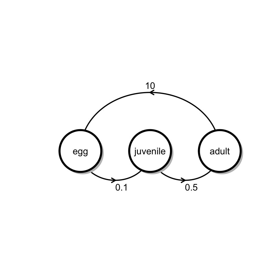
Consider a bird species where each (female) adult lays \(10\text{ eggs}\). Only \(10\%\) of eggs successfully hatch into juveniles, and \(50\%\) of juveniles survive and mature into adults. Adults die after reproduction.
Photo by Mike Erskine on Unsplash
Consider a short-lived plant that lives for 6 years. Each year, only \(1\%\) of seeds survive and germinate into seedlings. (The other seeds are eaten by squirrels and jays). \(50\%\) of seedlings survive to a juvenile stage, and \(95\%\) of juveniles transition into reproductive sub-adults. Each sub-adult makes \(10\text{ seeds}\) per year, and \(95\%\) of sub-adults transition into fully-mature adults. Each mature adult makes \(450\text{ seeds}\) per year, and \(10\%\) of adults survive to a post-reproductive adult stage, which are incapable of making new seeds.
These transition diagrams can be represented mathematically as transition matrices.
For a population with \(n\) stages, we can capture the demographic transitions in an \(n\mathrm{-by-}n\) matrix.
Consider a bird species where each (female) adult lays \(10\text{ eggs}\). Only \(10\%\) of eggs successfully hatch into juveniles, and \(50\%\) of juveniles survive and mature into adults. Adults die after reproduction.
\[ \begin{bmatrix} ~ & ~ & ~ & ~ & ~& ~ & ~ \\ ~ & ~ & ~ & ~ & ~& ~ & ~ \\ ~ & ~ & ~ & ~ & ~& ~ & ~ \\ ~ & ~ & ~ & ~ & ~& ~ & ~ \\ ~ & ~ & ~ & ~ & ~& ~ & ~ \\ ~ & ~ & ~ & ~ & ~& ~ & ~ \end{bmatrix} \]
Consider a bird species where each (female) adult lays \(10\text{ eggs}\). Only \(10\%\) of eggs successfully hatch into juveniles, and \(50\%\) of juveniles survive and mature into adults. Adults die after reproduction.
\[ \begin{bmatrix} 0 & 0 & 10 \\ 0.1 & 0 & 0 \\ 0 & 0.5 & 0 \end{bmatrix} \]
Your turn
Consider a species of fish whose individuals live for 3 years (age classes 0, 1, 2, and 3). Newborn fish have a \(30\%\) survival rate to year 1; year 1 fish have a \(80\%\) survival rate to year 2; year 2 fish have a \(50\%\) survival rate to year 3; and all fish die in their third year.
Newborn fish are sexually immature and cannot give birth. Year 1 fish can give birth to \(1\) newborn per year; Year 2 fish can give birth to \(8\) newborns per year; and Year 3 fish can only give birth to \(0.5\) newborns per year.
Draw a transition diagram and write the transition matrix for this population.
\[ \begin{bmatrix} 0 & 1 & 8 & 0.5 \\ 0.3 & 0 & 0 & 0 \\ 0 & 0.8 & 0 & 0 \\ 0 & 0 & 0.5 & 0 \end{bmatrix} \]
\[ \begin{bmatrix} 0 & 1 & 8 & 0.5 \\ 0.3 & 0 & 0 & 0 \\ 0 & 0.8 & 0 & 0 \\ 0 & 0 & 0.5 & 0 \end{bmatrix} \]
At time \(t=0\), the population has \(52\) individuals in stage 0, \(10\) in stage 1, \(15\) in stage 2, and \(30\) in stage 3.
What is the expected distribution of individuals at \(t=1\)?
Matrix product of the transition matrix and the current distribution:
\[ \begin{bmatrix} 0 & 1 & 8 & 0.5 \\ 0.3 & 0 & 0 & 0 \\ 0 & 0.8 & 0 & 0 \\ 0 & 0 & 0.5 & 0 \end{bmatrix} \times \begin{bmatrix} 52 \\ 10 \\ 16 \\ 30 \end{bmatrix} \]
Matrix product of the transition matrix and the current distribution:
\[ \begin{bmatrix} 0 & 1 & 8 & 0.5 \\ 0.3 & 0 & 0 & 0 \\ 0 & 0.8 & 0 & 0 \\ 0 & 0 & 0.5 & 0 \end{bmatrix} \times \begin{bmatrix} 52 \\ 10 \\ 16 \\ 30 \end{bmatrix} = \begin{bmatrix} 153 \\ 15 \\ 8 \\ 8 \end{bmatrix} \]
For timestep \(2\):
\[ \begin{bmatrix} 0 & 1 & 8 & 0.5 \\ 0.3 & 0 & 0 & 0 \\ 0 & 0.8 & 0 & 0 \\ 0 & 0 & 0.5 & 0 \end{bmatrix} \times \begin{bmatrix} 153 \\ 15 \\ 8 \\ 8 \end{bmatrix} \]
For timestep \(2\):
\[ \begin{bmatrix} 0 & 1 & 8 & 0.5 \\ 0.3 & 0 & 0 & 0 \\ 0 & 0.8 & 0 & 0 \\ 0 & 0 & 0.5 & 0 \end{bmatrix} \times \begin{bmatrix} 153 \\ 15 \\ 8 \\ 8 \end{bmatrix} = \begin{bmatrix} 83 \\ 45.9 \\ 12 \\ 4 \end{bmatrix} \]
For timestep \(3\):
\[ \begin{bmatrix} 0 & 1 & 8 & 0.5 \\ 0.3 & 0 & 0 & 0 \\ 0 & 0.8 & 0 & 0 \\ 0 & 0 & 0.5 & 0 \end{bmatrix} \times \begin{bmatrix} 83 \\ 45.9 \\ 12 \\ 4 \end{bmatrix} = \dots \]
\[ \begin{bmatrix} 0 & 1 & 8 & 0.5 \\ 0.3 & 0 & 0 & 0 \\ 0 & 0.8 & 0 & 0 \\ 0 & 0 & 0.5 & 0 \end{bmatrix} \xrightarrow[]{\text{Eigenvalue}} 1.33 \]
R