Population Ecology, pt 2:

Structured populations

Stage structured populations

Think back to the assumptions made in the simple exponential model of population growth (\(\frac{dN}{dt} = rN\)).

• Which assumption(s) are we relaxing when accounting for age/stage structure in populations?

Photo by Joshua J. Cotten on Unsplash

Monarch butterflies are migratory species that spend the North American winter in southwestern Mexico, and return to the US and Canada to breed during the summer months.

• The dynamics of these butterflies during the summer months is as follows (estimates from Hunt & Tongan 2017):

• Each female adult butterfly can lay up to \(45\) viable eggs, of which only \(3.4\%\) survive to the chrysalis stage. Eggs that make it to the chrysalis stage survive into the adult stage at rate of \(85\%\).

• Your task : Draw the life transition diagram and write the transition matrix for the monarch butterfly.

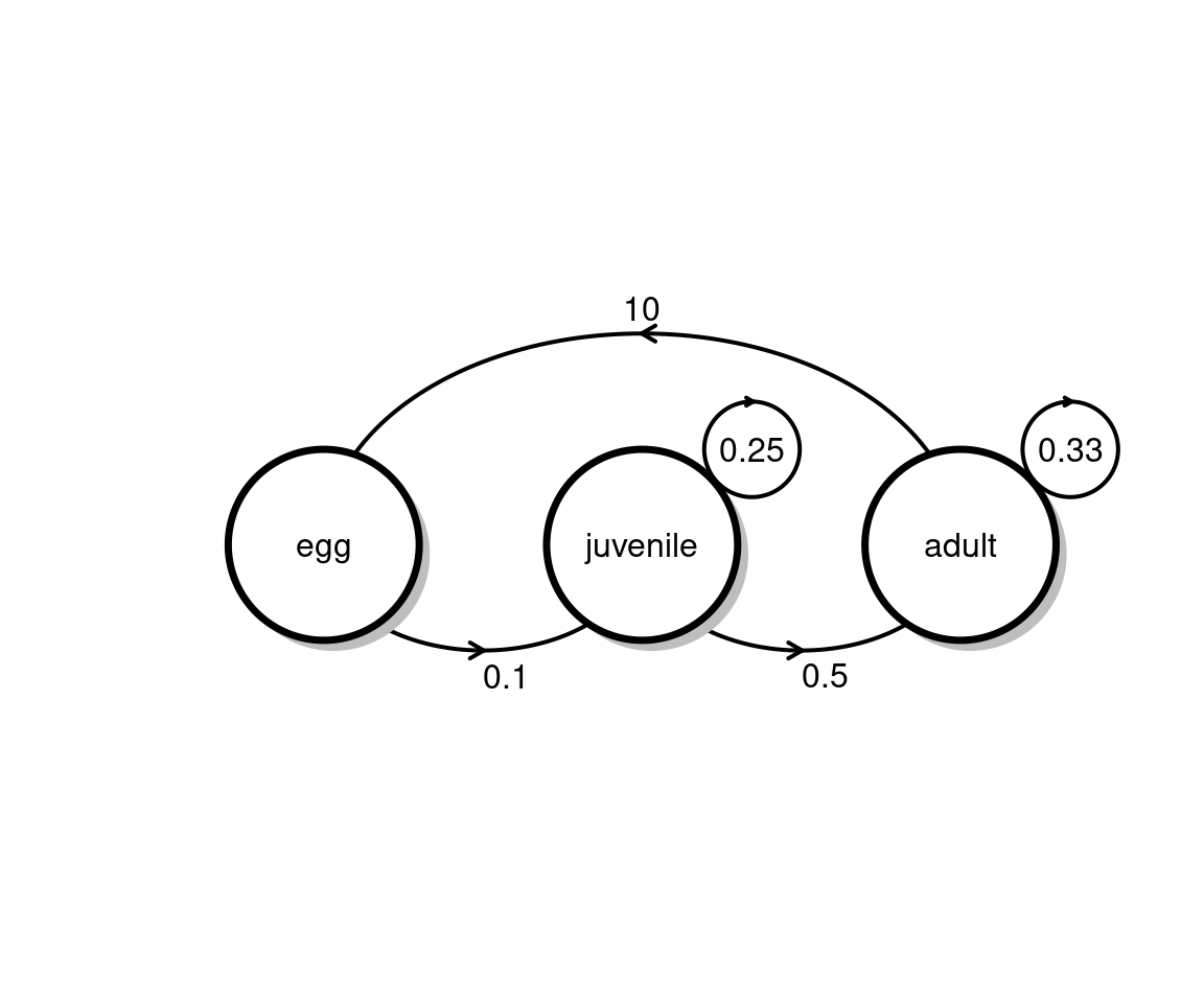
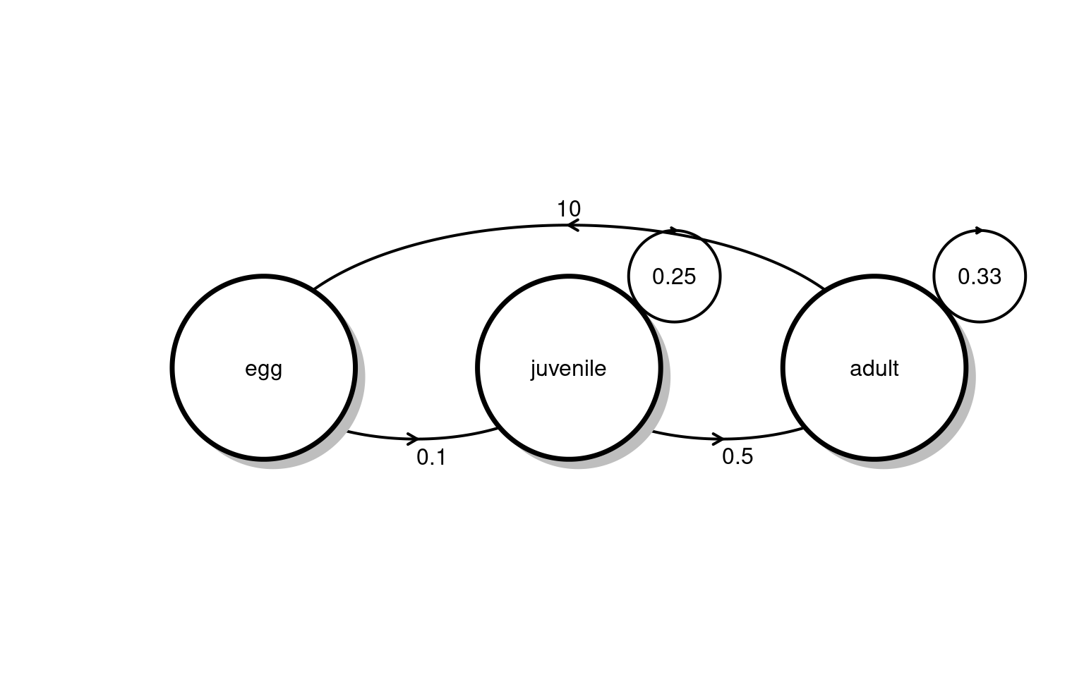
• Consider a species whose life cycle is described by the following matrix:

\[ \begin{bmatrix} 0 & 1 & 8 & 0.5 \\ 0.3 & 0 & 0 & 0 \\ 0 & 0.8 & 0 & 0 \\ 0 & 0 & 0.5 & 0 \end{bmatrix} \]

Draw a life transition diagram representing this matrix

Consider a species of fish whose individuals live for 3 years (age classes 0, 1, 2, and 3). Newborn fish have a \(30\%\) survival rate to year 1; year 1 fish have a \(80\%\) survival rate to year 2; year 2 fish have a \(50\%\) survival rate to year 3; and all fish die in their third year.

Newborn fish are sexually immature and cannot give birth. Year 1 fish can give birth to \(1\) newborn per year; Year 2 fish can give birth to \(8\) newborns per year; and Year 3 fish can only give birth to \(0.5\) newborns per year.

Structure of transition matrices

For a population with \(n\) stages, we can capture the demographic transitions in an \(n\mathrm{-by-}n\) matrix.

• Each element captures the contribution from the current column, to the current row.
  • The top row always reflects new births
  • The first (leftmost) column reflects the youngest individuals
  • The last (rightmost) column reflects the oldest individuals

The value of a transition matrix

• The product of the current population distribution and the transition matrix tells you the future population distribution

The value of a transition matrix

• From our worked example, recall the transition matrix

\[ \begin{bmatrix} 0 & 1 & 8 & 0.5 \\ 0.3 & 0 & 0 & 0 \\ 0 & 0.8 & 0 & 0 \\ 0 & 0 & 0.5 & 0 \end{bmatrix} \]

• At time \(t=0\), the population has \(52\) individuals in stage 0, \(10\) in stage 1, \(15\) in stage 2, and \(30\) in stage 3.

• What is the expected distribution of individuals at \(t=1\)?

The value of a transition matrix

Matrix product of the transition matrix and the current distrubition:

\[ \begin{bmatrix} 0 & 1 & 8 & 0.5 \\ 0.3 & 0 & 0 & 0 \\ 0 & 0.8 & 0 & 0 \\ 0 & 0 & 0.5 & 0 \end{bmatrix} \times \begin{bmatrix} 52 \\ 10 \\ 16 \\ 30 \end{bmatrix} \]

The value of a transition matrix

Matrix product of the transition matrix and the current distrubition:

\[ \begin{bmatrix} 0 & 1 & 8 & 0.5 \\ 0.3 & 0 & 0 & 0 \\ 0 & 0.8 & 0 & 0 \\ 0 & 0 & 0.5 & 0 \end{bmatrix} \times \begin{bmatrix} 52 \\ 10 \\ 16 \\ 30 \end{bmatrix} = \begin{bmatrix} 153 \\ 15 \\ 8 \\ 8 \end{bmatrix} \]

The value of a transition matrix

For timestep \(2\):

\[ \begin{bmatrix} 0 & 1 & 8 & 0.5 \\ 0.3 & 0 & 0 & 0 \\ 0 & 0.8 & 0 & 0 \\ 0 & 0 & 0.5 & 0 \end{bmatrix} \times \begin{bmatrix} 153 \\ 15 \\ 8 \\ 8 \end{bmatrix} \]

The value of a transition matrix

For timestep \(2\):

\[ \begin{bmatrix} 0 & 1 & 8 & 0.5 \\ 0.3 & 0 & 0 & 0 \\ 0 & 0.8 & 0 & 0 \\ 0 & 0 & 0.5 & 0 \end{bmatrix} \times \begin{bmatrix} 153 \\ 15 \\ 8 \\ 8 \end{bmatrix} = \begin{bmatrix} 83 \\ 45.9 \\ 12 \\ 4 \end{bmatrix} \]

The value of a transition matrix

For timestep \(3\):

\[ \begin{bmatrix} 0 & 1 & 8 & 0.5 \\ 0.3 & 0 & 0 & 0 \\ 0 & 0.8 & 0 & 0 \\ 0 & 0 & 0.5 & 0 \end{bmatrix} \times \begin{bmatrix} 83 \\ 45.9 \\ 12 \\ 4 \end{bmatrix} = \dots \]

The value of a transition matrix

• We can keep iterating over and over (and over), or….
• Calculate the \(\mathrm{eigenvalue}\) of the transition matrix
• The dominant eigenvalue reflects the long-term growth rate.

\[ \begin{bmatrix} 0 & 1 & 8 & 0.5 \\ 0.3 & 0 & 0 & 0 \\ 0 & 0.8 & 0 & 0 \\ 0 & 0 & 0.5 & 0 \end{bmatrix} \xrightarrow[]{\text{Eigenvalue}} 1.33 \]

The value of a transition matrix

• The dominant Eigenvalue represents the expected long-term annual growth rate (\(\lambda\))
• Populations grow when \(\lambda \gt 1\)
• Populations shrink when \(\lambda \lt 1\)
• Population size is stable when \(\lambda = 1\)

For more on what Eigenvalues are…

Check out this video.

What happens when transition rates change?

• Let’s return to our previous fish example. In normal conditions, newborn fish have a \(30\%\) survival rate to year 1; year 1 fish have a \(80\%\) survival rate to year 2; year 2 fish have a \(50\%\) survival rate to year 3; and all fish die in their third year.

• An extreme heat event causes newborn survival rates to plummet to \(0%\) in a given year. What are the consequences for the population?

What happens when transition rates change?

\[ \begin{bmatrix} 0 & 1 & 8 & 0.5 \\ 0.3 & 0 & 0 & 0 \\ 0 & 0.8 & 0 & 0 \\ 0 & 0 & 0.5 & 0 \end{bmatrix} \]

\[ \begin{bmatrix} 0 & 1 & 8 & 0.5 \\ 0.3 \to 0 & 0 & 0 & 0 \\ 0 & 0.8 & 0 & 0 \\ 0 & 0 & 0.5 & 0 \end{bmatrix} \]

What happens when transition rates change?

• What if instead, the extreme heat event only reduced newborn survival from \(30%\) to \(20\%\)?

• Or if newborn rates were unaffected, but survival from year 1 to 2 was reduced from \(80\%\) to \(70\%\)?

\[ \begin{bmatrix} 0 & 1 & 8 & 0.5 \\ 0.3 \to 0.2 & 0 & 0 & 0 \\ 0 & 0.8 & 0 & 0 \\ 0 & 0 & 0.5 & 0 \end{bmatrix} \]

\[ \begin{bmatrix} 0 & 1 & 8 & 0.5 \\ 0.3 \to 0.2 & 0 & 0 & 0 \\ 0 & 0.8 & 0 & 0 \\ 0 & 0 & 0.5 & 0 \end{bmatrix} \Rightarrow \lambda = 1.15 \]

\[ \begin{bmatrix} 0 & 1 & 8 & 0.5 \\ 0.3 & 0 & 0 & 0 \\ 0 & 0.8 \to 0.7 & 0 & 0 \\ 0 & 0 & 0.5 & 0 \end{bmatrix} \]

\[ \begin{bmatrix} 0 & 1 & 8 & 0.5 \\ 0.3 & 0 & 0 & 0 \\ 0 & 0.8 \to 0.7 & 0 & 0 \\ 0 & 0 & 0.5 & 0 \end{bmatrix} \Rightarrow \lambda = 1.28 \]

The value of a transition matrix

How is the growth rate affected by particular transitions?

\[ \begin{bmatrix} 0 & 1 & 8 & 0.5 \\ 0.3 \to 0.2 & 0 & 0 & 0 \\ 0 & 0.8 & 0 & 0 \\ 0 & 0 & 0.5 & 0 \end{bmatrix} \Rightarrow \lambda = \boxed{1.33 \Rightarrow 1.15} \]

\[ \begin{bmatrix} 0 & 1 & 8 & 0.5 \\ 0.3 & 0 & 0 & 0 \\ 0 & 0.8 \to 0.7 & 0 & 0 \\ 0 & 0 & 0.5 & 0 \end{bmatrix} \Rightarrow \lambda = \boxed{1.33 \Rightarrow 1.28} \]

We can go through each entry one-by-one and identify critical transitions (Sensitivity analysis)

The value of a transition matrix

This could also go the other way– increase in \(\lambda\)

\[ \begin{bmatrix} 0 & 1 & 8 & 0.5 \\ 0.3 \to 0.4 & 0 & 0 & 0 \\ 0 & 0.8 & 0 & 0 \\ 0 & 0 & 0.5 & 0 \end{bmatrix} \Rightarrow \lambda = \boxed{1.33 \Rightarrow 1.47} \]

\[ \begin{bmatrix} 0 & 1 & 8 & 0.5 \\ 0.3 & 0 & 0 & 0 \\ 0 & 0.8 \to 0.9 & 0 & 0 \\ 0 & 0 & 0.5 & 0 \end{bmatrix} \Rightarrow \lambda = \boxed{1.33 \Rightarrow 1.38} \]

We can go through each entry one-by-one and identify critical transitions (Sensitivity analysis)

But there is a problem…

• Increasing one parameter by 0.1 might not be equivalent to increasing another by the same amount.

\[ \begin{bmatrix} 0 & 1 & 8 & 0.5 \\ 0.3 \to 0.4 & 0 & 0 & 0 \\ 0 & 0.8 & 0 & 0 \\ 0 & 0 & 0.5 & 0 \end{bmatrix} \]

\[ \begin{bmatrix} 0 & 1 & 8 & 0.5 \\ 0.3 & 0 & 0 & 0 \\ 0 & 0.8 \to 0.9 & 0 & 0 \\ 0 & 0 & 0.5 & 0 \end{bmatrix} \]

Elasticity analysis

Quantify the effects of proportional changes

\[ \begin{bmatrix} 0 & 1 & 8 & 0.5 \\ 0.3 \to 0.27 & 0 & 0 & 0 \\ 0 & 0.8 & 0 & 0 \\ 0 & 0 & 0.5 & 0 \end{bmatrix} \]

\[ \begin{bmatrix} 0 & 1 & 8 & 0.5 \\ 0.3 & 0 & 0 & 0 \\ 0 & 0.8 \to 0.72 & 0 & 0 \\ 0 & 0 & 0.5 & 0 \end{bmatrix} \]

Elasticity analysis

Quantify the effects of proportional changes

\[ \begin{bmatrix} 0 & 1 & 8 & 0.5 \\ 0.3 \to 0.27 & 0 & 0 & 0 \\ 0 & 0.8 & 0 & 0 \\ 0 & 0 & 0.5 & 0 \end{bmatrix} \Rightarrow \lambda= \boxed{1.33 \Rightarrow 1.28} \]

\[ \begin{bmatrix} 0 & 1 & 8 & 0.5 \\ 0.3 & 0 & 0 & 0 \\ 0 & 0.8 \to 0.72 & 0 & 0 \\ 0 & 0 & 0.5 & 0 \end{bmatrix} \Rightarrow \lambda = \boxed{1.33 \Rightarrow 1.29} \]

Elasticity analysis

Quantify the effects of proportional changes

\[ \begin{bmatrix} 0 & 1 & 8 & 0.5 \\ 0.3 \to 0.33 & 0 & 0 & 0 \\ 0 & 0.8 & 0 & 0 \\ 0 & 0 & 0.5 & 0 \end{bmatrix} \Rightarrow \lambda= \boxed{1.33 \Rightarrow 1.38} \]

\[ \begin{bmatrix} 0 & 1 & 8 & 0.5 \\ 0.3 & 0 & 0 & 0 \\ 0 & 0.8 \to 0.88 & 0 & 0 \\ 0 & 0 & 0.5 & 0 \end{bmatrix} \Rightarrow \lambda = \boxed{1.33 \Rightarrow 1.37} \]

Age vs. stage-based matrices

• So far, we have conflated age and stage (e.g. “1-year-old” == “Juvenile”, “2-year-old” == “Subadult”, etc.)

• But, there’s a potential issue – e.g. what if the juvenile stage extends for multiple year?

Empirical application:
Population dynamics of red cockaded woodpeckers

(a) Red bellied

(b) Red headed

(c) Downy

(d) Hairy

Figure 1: Some common woodpeckers around Baton Rouge (photos from All About Birds)

Red cockaded woodpeckers: an uncommon (near threatened) species

Causes for the decline

From Ziegler & Walter 2014, in Ecological Applications

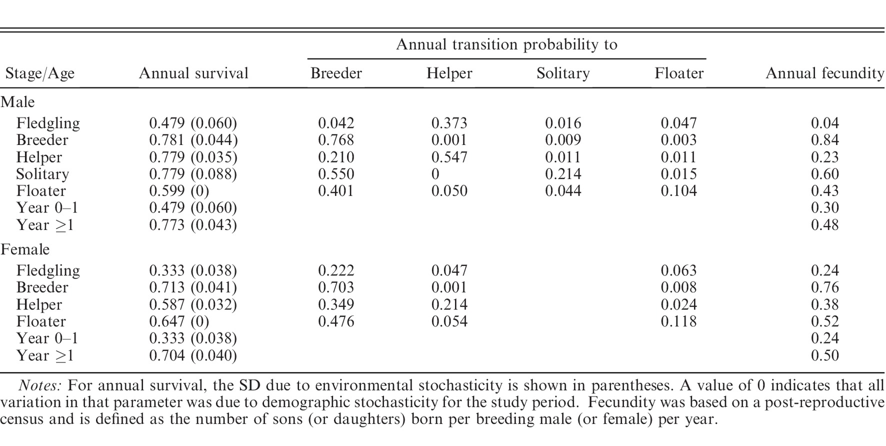
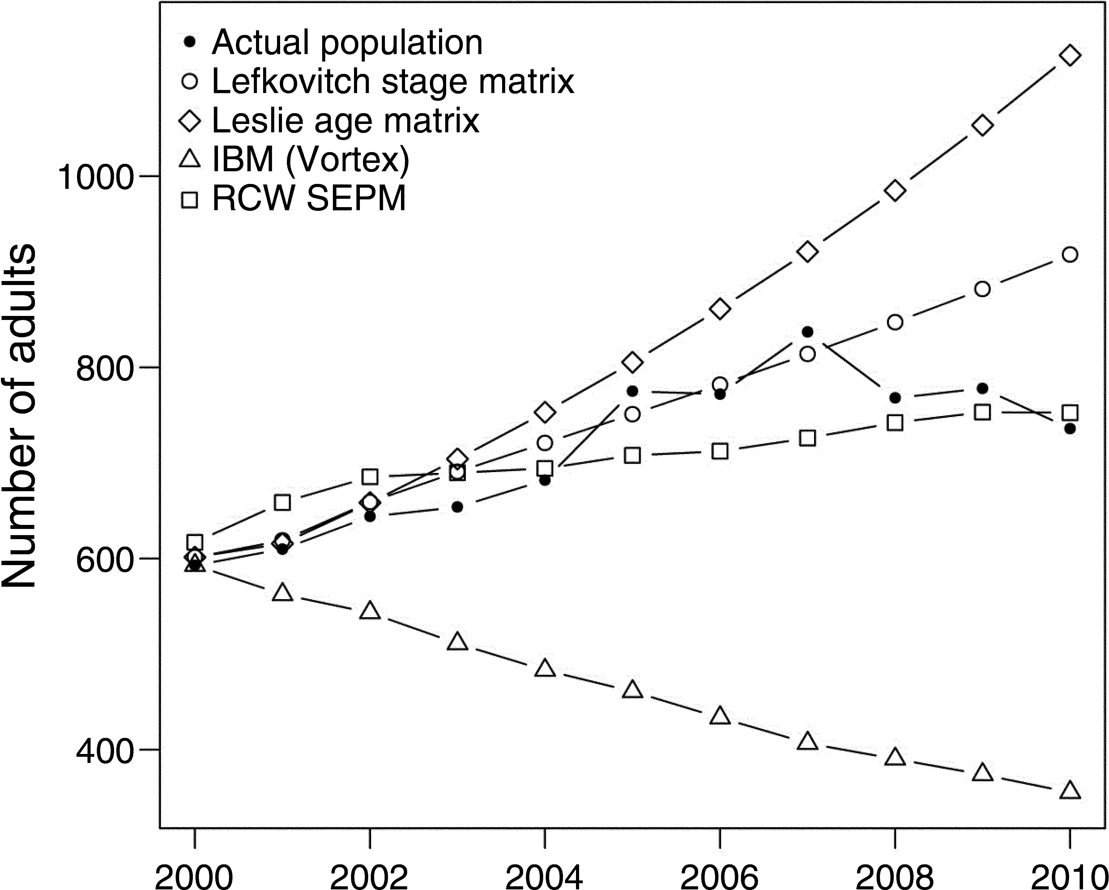
The Red Cockaded Woodpecker is an endangered species endemic to fire dependent longleaf pine ecosystems in the southeastern United States. Primary threats to the species include a lack of suitable cavity trees, habitat fragmentation, and fire suppression that results in hardwood midstory encroachment and the declining suitability of foraging habitat.

Preferred habitat for the species consists of mature, open pine forest with large trees, sparse midstory, and a lush herbaceous ground cover, conditions primarily maintained through frequent, low-intensity ground fires. Old pines are an especially important part of RCW ecology because RCWs construct cavities in living trees, and heartwood diameter is a function of age. Cavity construction is difficult and time intensive, and RCW groups will defend and use the same cavity trees for many years

Photo by Gaurav Kandlikar near Abita Springs

How to build a matrix population model for RCW?

Question 1: What are the stages?

RCWs are territorial and cooperatively breeding with a complex social structure.

Groups are composed of a monogamous breeding pair and non-breeding helpers.

Fledglings either remain on the natal territory as helpers or disperse

Almost all females disperse in either the fall or spring following fledging and ultimately obtain breeding positions if they survive, although they may act as floaters before acquiring a breeding opportunity.

Substantial numbers of male fledglings stay as helpers, and those that survive ultimately inherit the breeding position in their natal territory or fill breeding vacancies in neighboring territories. Other male fledglings disperse to either become breeders, solitary males, floaters, or (to a lesser extent) helpers in another territory

So… what are the stages? It’s complex!

So… what are the stages? It’s complex!

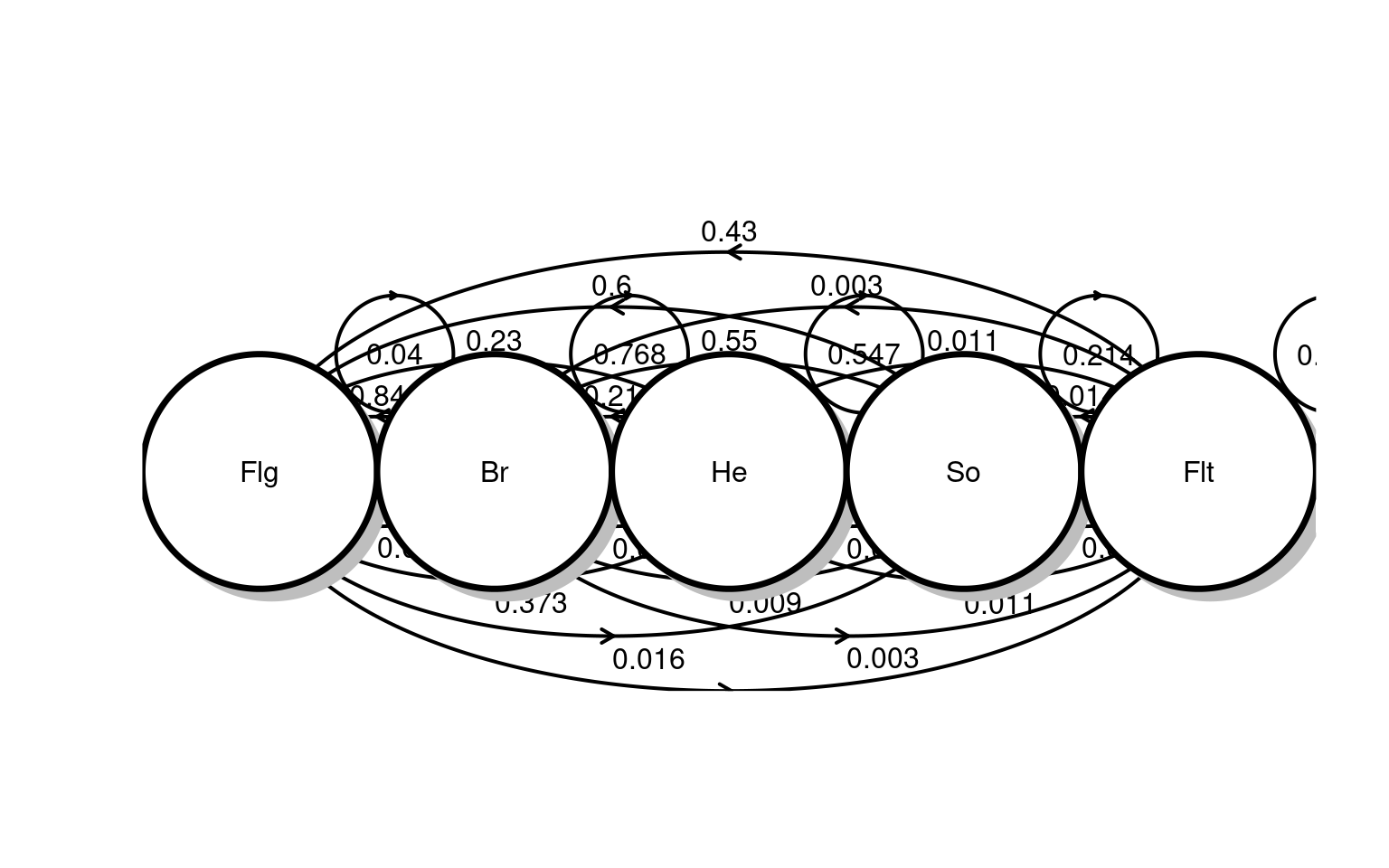
Banded individuals were classified according to age and stage class each year, with potential stage classes including fledglings, individuals <1 year old; breeders, males and females that occupy a territory and have the potential to produce offspring; helpers, nonbreeding adults that are part of the social group and assist breeders; solitary males, adult males that maintain a territory but are unpaired and do not breed; and floaters, adults without territories that do not breed

Question 2: What are the transition rates and reproduction rates?

Question 3: How to put these together into a matrix?

As in Heppell et al. (1994), matrices were constructed in this study as male-only models because, unlike females, males almost exclusively comprise the helper class and can hold territories despite being unpaired

Simplified example

• Consider the example from last week:

\[ \begin{bmatrix} 0 & 0 & 10 \\ 0.1 & 0 & 0 \\ 0 & 0.5 & 0 \end{bmatrix} \]

Simplified example

• Now, consider what happens when individuals can persist in a given stage.
• Juveniles stay juveniles at a rate of 0.25, adults stay adults at a rate of 0.33

\[ \begin{bmatrix} 0 & 0 & 10 \\ 0.1 & 0 \to 0.25 & 0 \\ 0 & 0.5 & 0 \to 0.33 \end{bmatrix} \]

$arr
   row col Angle Value      rad    ArrowX       ArrowY TextX      TextY
1    1   1   NaN  0.04 0.106962 0.2166801 7.208729e-01 0.215  0.6139241
2    2   1     0 0.042 0.100000 0.1995288 3.000011e-01 0.200  0.2800000
3    3   1     0 0.373 0.200000 0.2990575 2.000022e-01 0.300  0.1800000
4    4   1     0 0.016 0.300000 0.3985863 1.000033e-01 0.400  0.0800000
5    5   1     0 0.047 0.400000 0.4981151 4.441314e-06 0.500 -0.0200000
6    1   2     0  0.84 0.100000 0.2001571 4.999999e-01 0.200  0.5200000
7    2   2   NaN 0.768 0.106962 0.4166801 7.208729e-01 0.415  0.6139241
8    3   2     0 0.001 0.100000 0.3995288 3.000011e-01 0.400  0.2800000
9    4   2     0 0.009 0.200000 0.4990575 2.000022e-01 0.500  0.1800000
10   5   2     0 0.003 0.300000 0.5985863 1.000033e-01 0.600  0.0800000
11   1   3     0  0.23 0.200000 0.3003142 5.999998e-01 0.300  0.6200000
12   2   3     0  0.21 0.100000 0.4001571 4.999999e-01 0.400  0.5200000
13   3   3   NaN 0.547 0.106962 0.6166801 7.208729e-01 0.615  0.6139241
14   4   3     0 0.011 0.100000 0.5995288 3.000011e-01 0.600  0.2800000
15   5   3     0 0.011 0.200000 0.6990575 2.000022e-01 0.700  0.1800000
16   1   4     0   0.6 0.300000 0.4004712 6.999996e-01 0.400  0.7200000
17   2   4     0  0.55 0.200000 0.5003142 5.999998e-01 0.500  0.6200000
18   4   4   NaN 0.214 0.106962 0.8166801 7.208729e-01 0.815  0.6139241
19   5   4     0 0.044 0.100000 0.7995288 3.000011e-01 0.800  0.2800000
20   1   5     0  0.43 0.400000 0.5006283 7.999995e-01 0.500  0.8200000
21   2   5     0 0.003 0.300000 0.6004712 6.999996e-01 0.600  0.7200000
22   3   5     0 0.011 0.200000 0.7003142 5.999998e-01 0.700  0.6200000
23   4   5     0 0.014 0.100000 0.8001571 4.999999e-01 0.800  0.5200000
24   5   5   NaN 0.104 0.106962 1.0166801 7.208729e-01 1.015  0.6139241

$comp
       x   y
[1,] 0.1 0.4
[2,] 0.3 0.4
[3,] 0.5 0.4
[4,] 0.7 0.4
[5,] 0.9 0.4

$radii
       x         y
[1,] 0.1 0.2139241
[2,] 0.1 0.2139241
[3,] 0.1 0.2139241
[4,] 0.1 0.2139241
[5,] 0.1 0.2139241

$rect
     xleft      ybot xright      ytop
[1,]   0.0 0.1860759    0.2 0.6139241
[2,]   0.2 0.1860759    0.4 0.6139241
[3,]   0.4 0.1860759    0.6 0.6139241
[4,]   0.6 0.1860759    0.8 0.6139241
[5,]   0.8 0.1860759    1.0 0.6139241

Many potential options

• What biology to include? What to exclude?

Which model to choose?

Takeaways

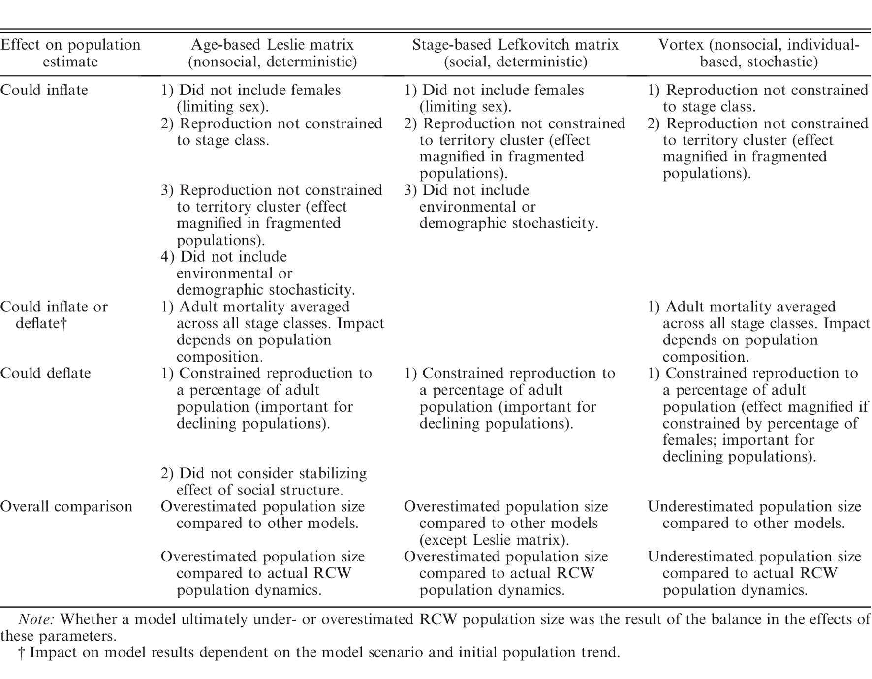
• Matrix population models as important tools for conservation and restoration

• Importance of comparing models that incorporate different aspects of a species’ biology

• Importance (and difficulty!) of collecting field data

• Integrating data with models enables predictions

More on Matrix models for informing conservation decisions

Small-group discussion

• Within each group, assign roles:
  • Timekeeper (Make sure everyone is contributing and group is addressing all questions)
  • Recorder (Take notes on the conversation)
  • Questioner (What were some points of confusion/clarification?)
  • Reporter (Responsible for sharing group discussion w/ class)

Small group discussion

1. What is the relationship between the Eigenvalue of a population transition matrix (\(\lambda\)) and the intrinsic growth parameter \(r\) we explored in the exponential growth model? What happens when \(\lambda = 1\)? What happens when \(r = 1\)?

2. The authors choose to construct a stage-based matrix rather than an age-based population matrix. Why? How did the authors get data to construct the matrix?

3. Table 4 of the paper provides the values for the loggerhead transition matrix. Draw this as a transition diagram.

4. Consider Figure 1 of the paper, and address the following questions:

• What is the name of the type of analysis that the authors conducted to create this figure? What does this analysis entail?
• What do the X- and Y-axis of the two panels represent?
• What is the takeaway from Panel B?

5. The authors consider several management scenarios that would enable \(\lambda\) to reach a value of 1 or more. Biologically, why is this threshold relevant, and what do the authors find is the most likely way to achieve this goal?

Population ecology review

Main themes of the unit so far:

• Measuring population sizes
• Dynamics of exponential growth
• Stage–structured populations

Measuring population sizes

• Here, we were exploring the challenges in what might be one of the most basic tasks of an ecologist: Counting the number of individuals in a population.
• We introduced the mark–recapture method as an approach for estimating population sizes
• We discussed how these estimates provide us an approximation of nature, and how we can improve our approximations

Tracking population growth

Part 1: exponential growth dynamics

• Predicting whether a population will grow, shrink, or stay stable is the next most pressing question.
• The simplest model of population growth assumes that populations only change by births and deaths
• Difference between birth and death rate gives the population growth rate \(r\).
• Populations grow if \(r>0\), or shrink if \(r<0\).

Tracking population growth

Part 2: Structured growth dynamics

• What if not all individuals are equally likely to die or reproduce?
• Matrices can capture a lot of biological detail about birth and death rates of individuals of different ages (or stages)
• Eigen-analysis tells us whether populations are expected to grow or shrink
• Elasticity analyses help us identify the most “impactful” life stages

In-class activity instructions

• Work on the activity independently for 15 minutes.
• Discuss with neighbors or in small groups for 5 minutes, during which you can revise any answers
  • I’d prefer if you don’t erase anything, just cross out things you are changing
• We will go over it together as a group afterwards.