Limits to population growth
Exponential and stage-structured population growth
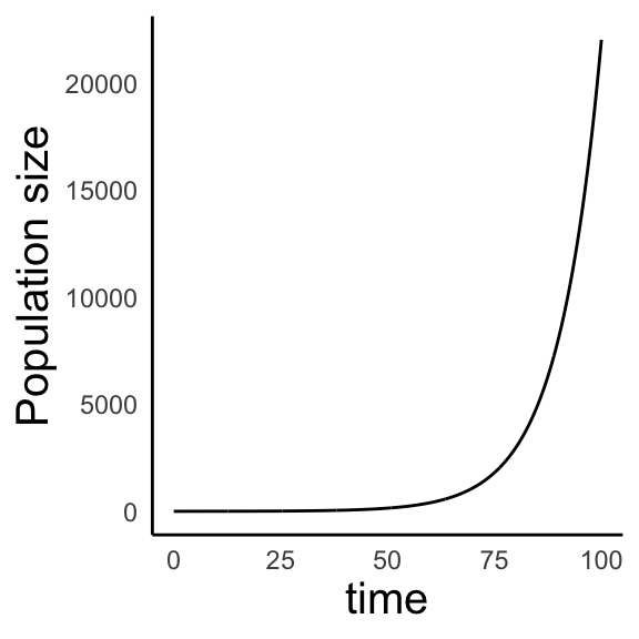
Exponential growth
\[\frac{dN}{dt} = rN\]
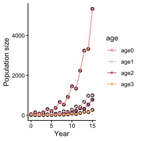
Stage-structured growth
\[N_{t+1} = \text{[transition matrix]} ~x~ \\ \text{[population vector]}\]
So far, we assumed constant birth and death rate (\(b\) and \(d\) don’t vary with \(N\))
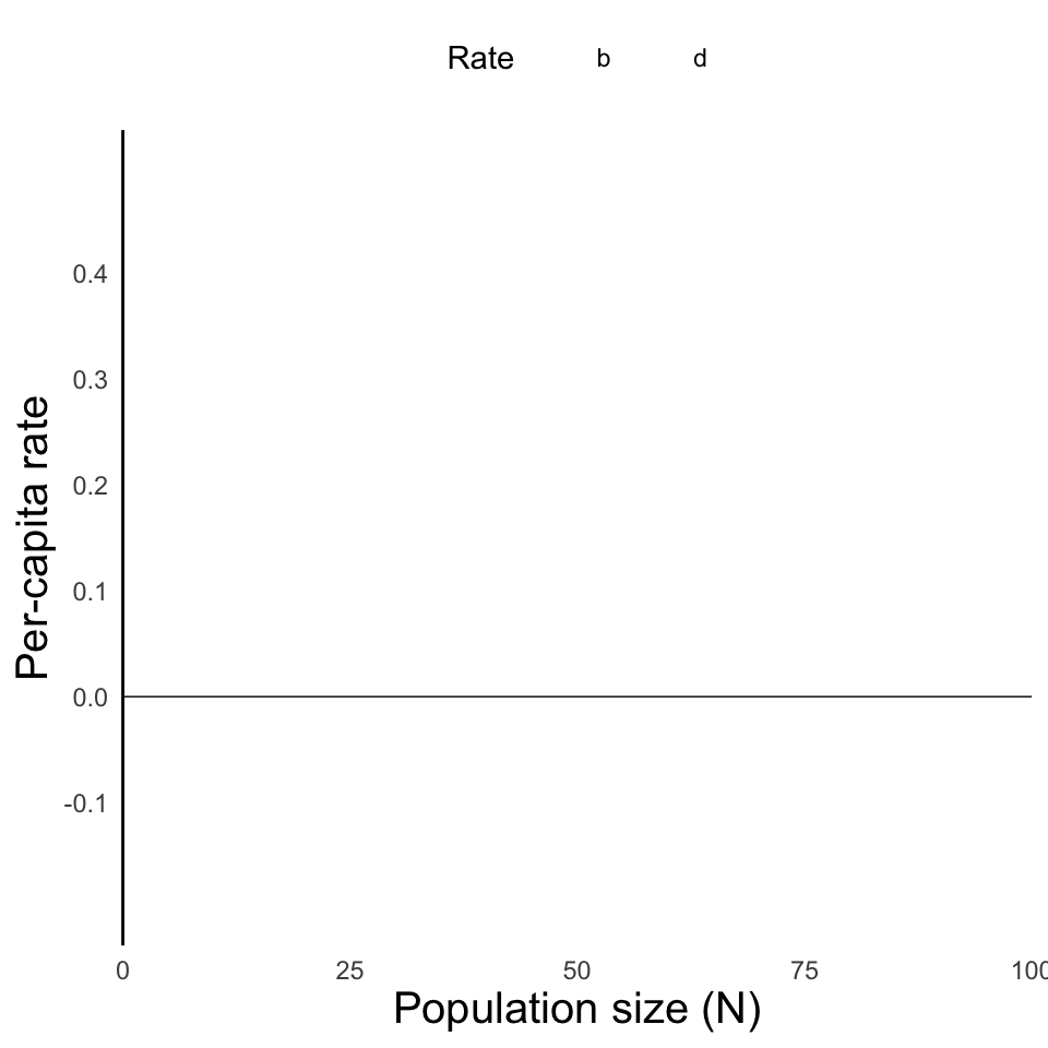
So far, we assumed constant birth and death rate (\(b\) and \(d\) don’t vary with \(N\))
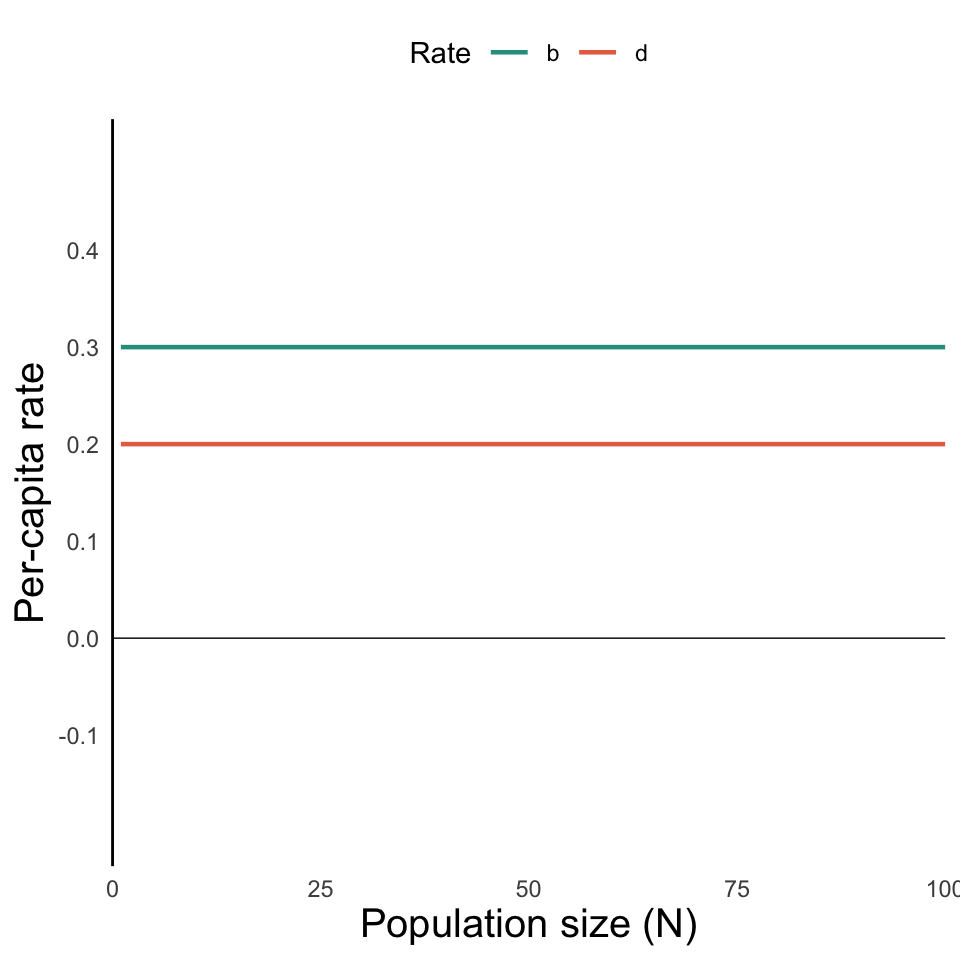
So far, we assumed constant birth and death rate (\(b\) and \(d\) don’t vary with \(N\))
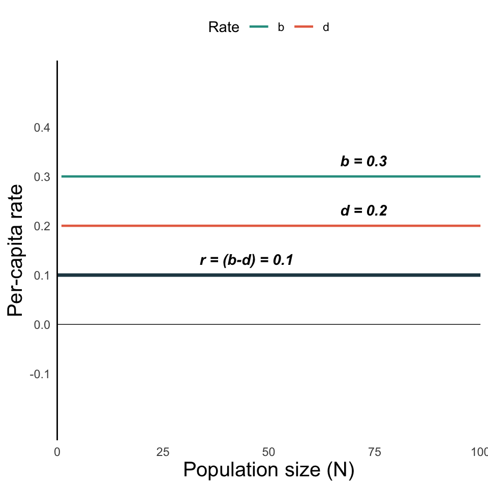
What if \(b\) and \(d\) are not constant?
We can easily imagine scenarios in which birth and death rates vary with population size.
- In social species (bees, ants, wolves, some woodpeckers, etc.), birth rates (\(b\)) might increase with population size
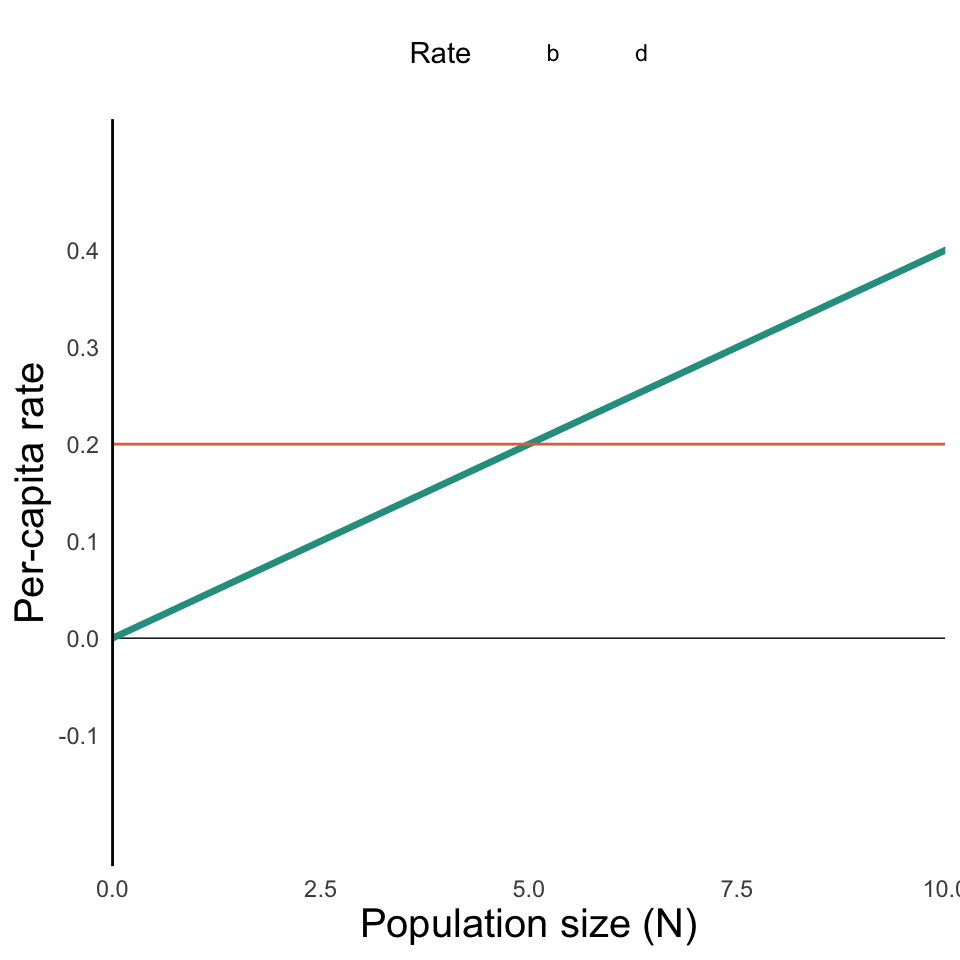
What if \(b\) and \(d\) are not constant?
We can easily imagine scenarios in which birth and death rates vary with population size.
- Under strict resource limitation, mortality rate might increase with population size
- Could also happen without resource limitation, e.g. higher rates of disease spread
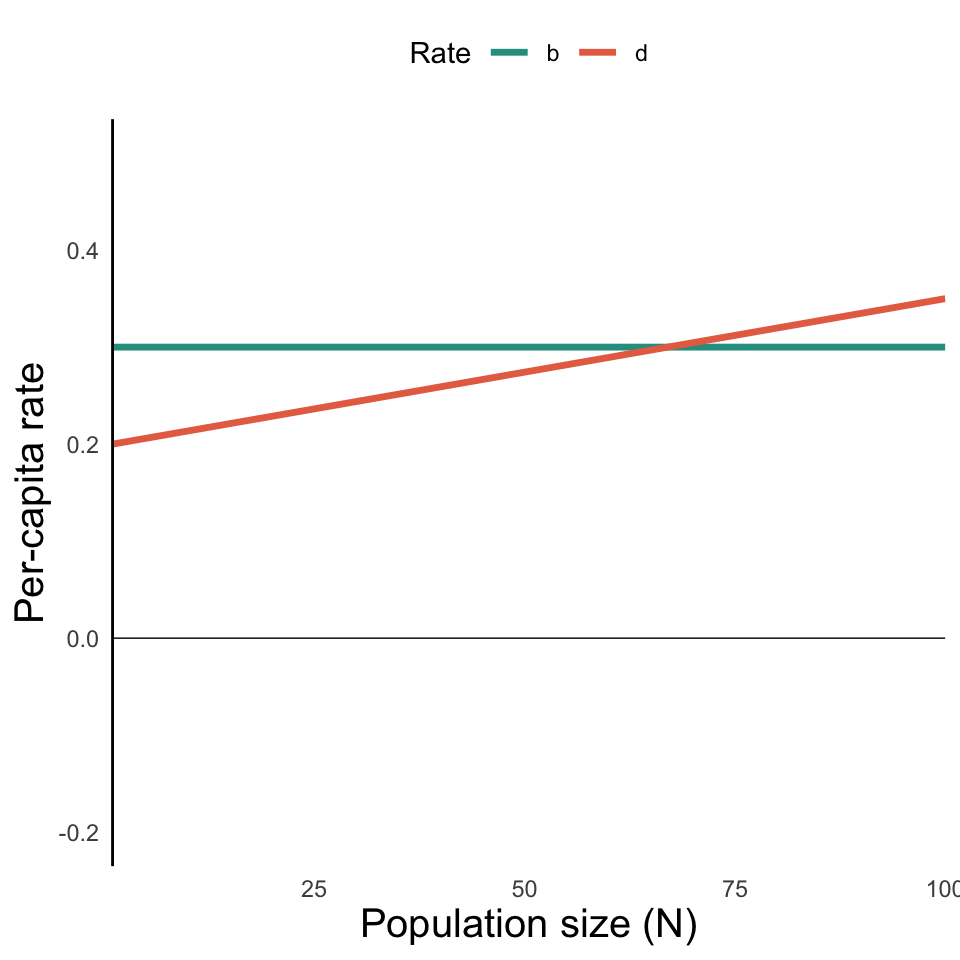
- Under this assumption (\(d\) increases with \(N\)), we see that there is a point at which \(\text{growth rate} = 0\).
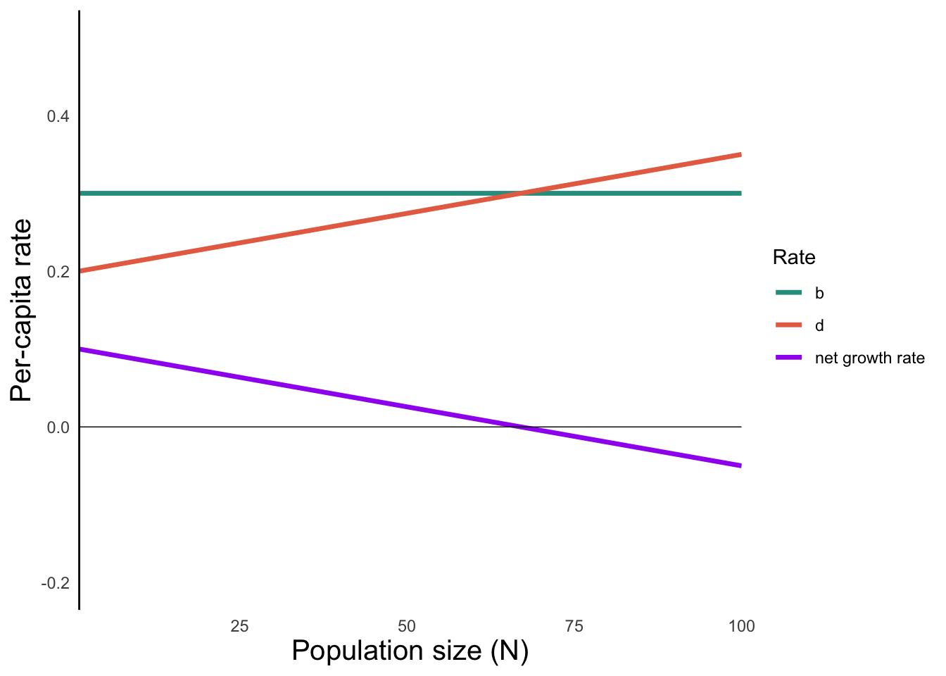
- \(r\) is the growth rate when \(N = 0\)
What happens when \(b-d = 0\)?
- Birth rate equals death rate
- No change in population size
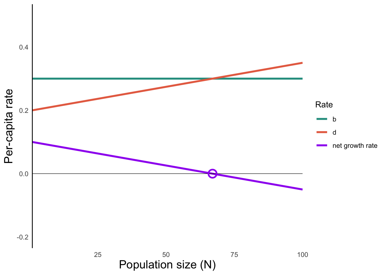
- The population size (\(N\)) at which growth rate equals zero is called the carrying capacity (\(K\))
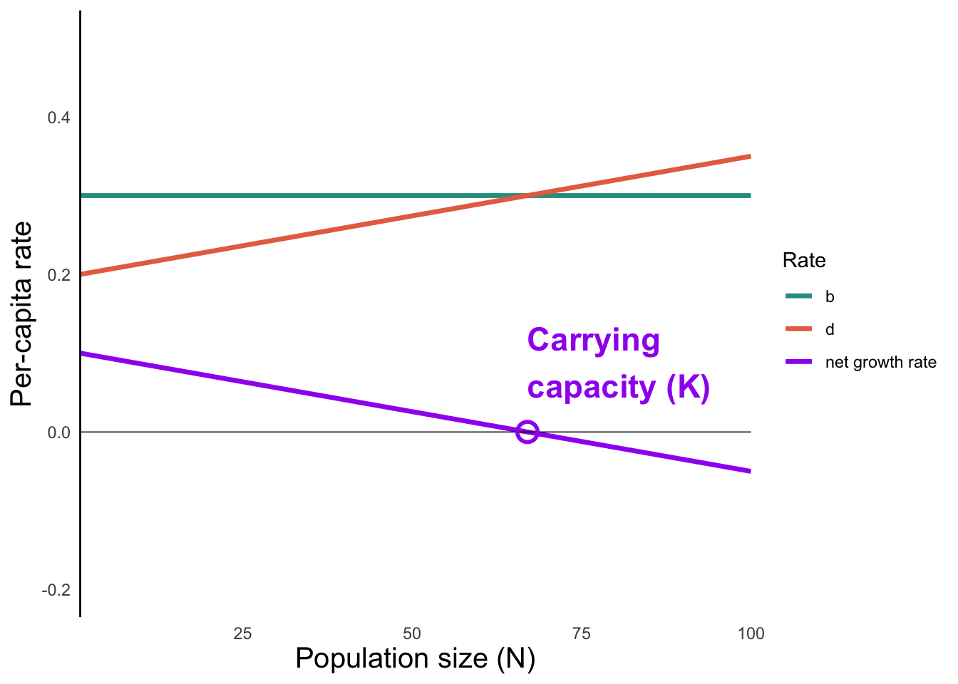
The population size (\(N\)) at which growth rate equals zero is called the carrying capacity (\(K\))
The population’s growth rate at \(N = 0\) is \(r\)
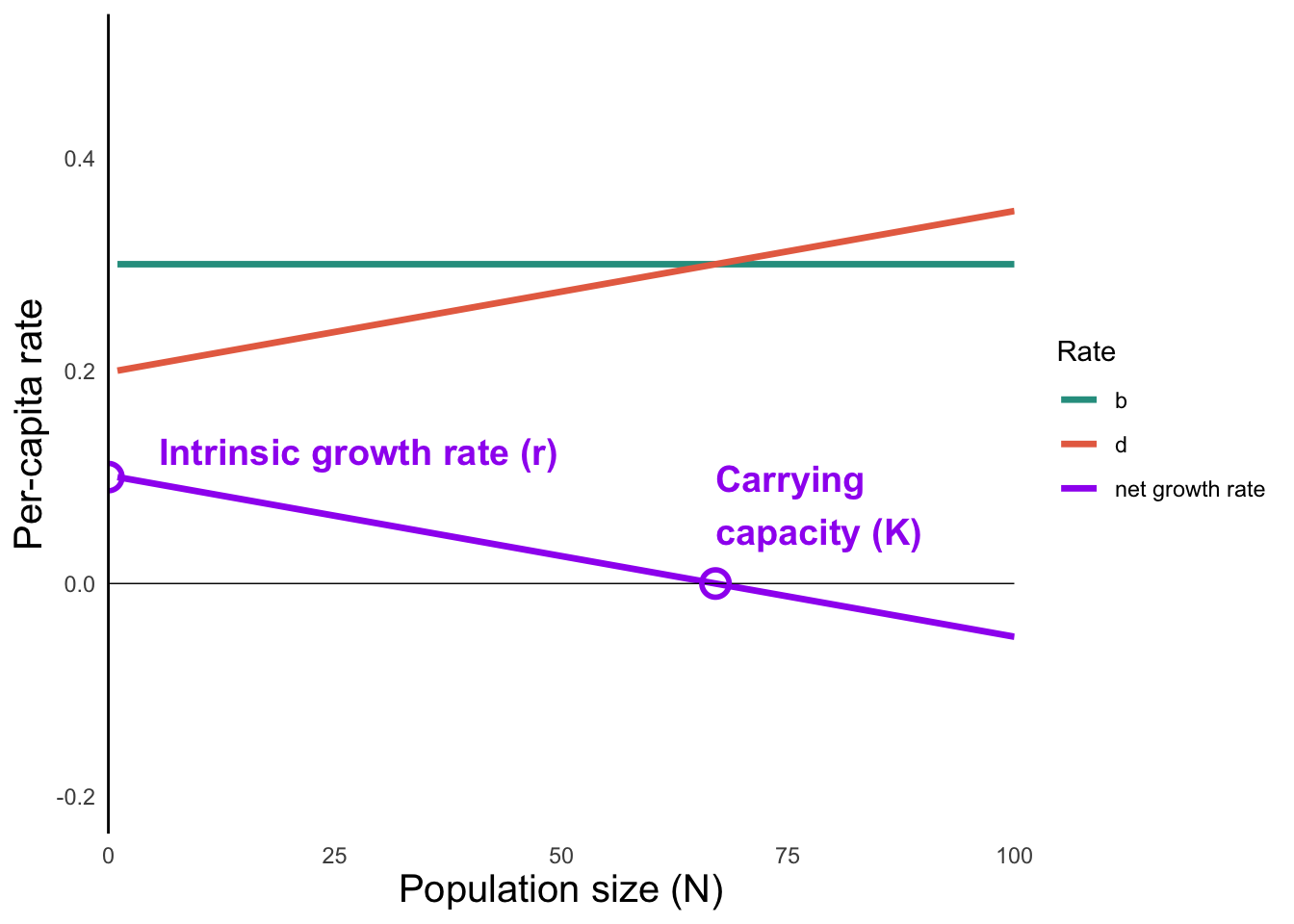
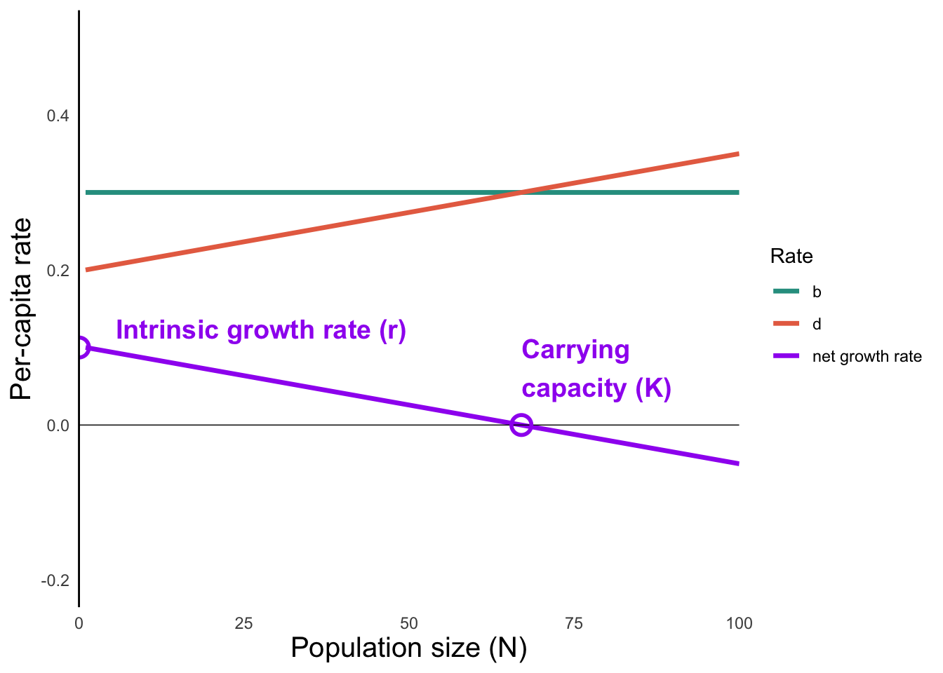
- The per-capita population growth rate (\(\frac{1}{N}\frac{dN}{dt}\)) for a population of a given size is the Y-axis value.
- The closer a population is to \(N = 0\), the closer its actual growth rate is to \(r\)
- The closer a population is to \(N = K\), the closer its actual growth rate is to \(0\)
- Populations that are bigger than K have negative population growth (until they fall back to carrying capacity)
Mathematical expression
What is the equation of the purple line?
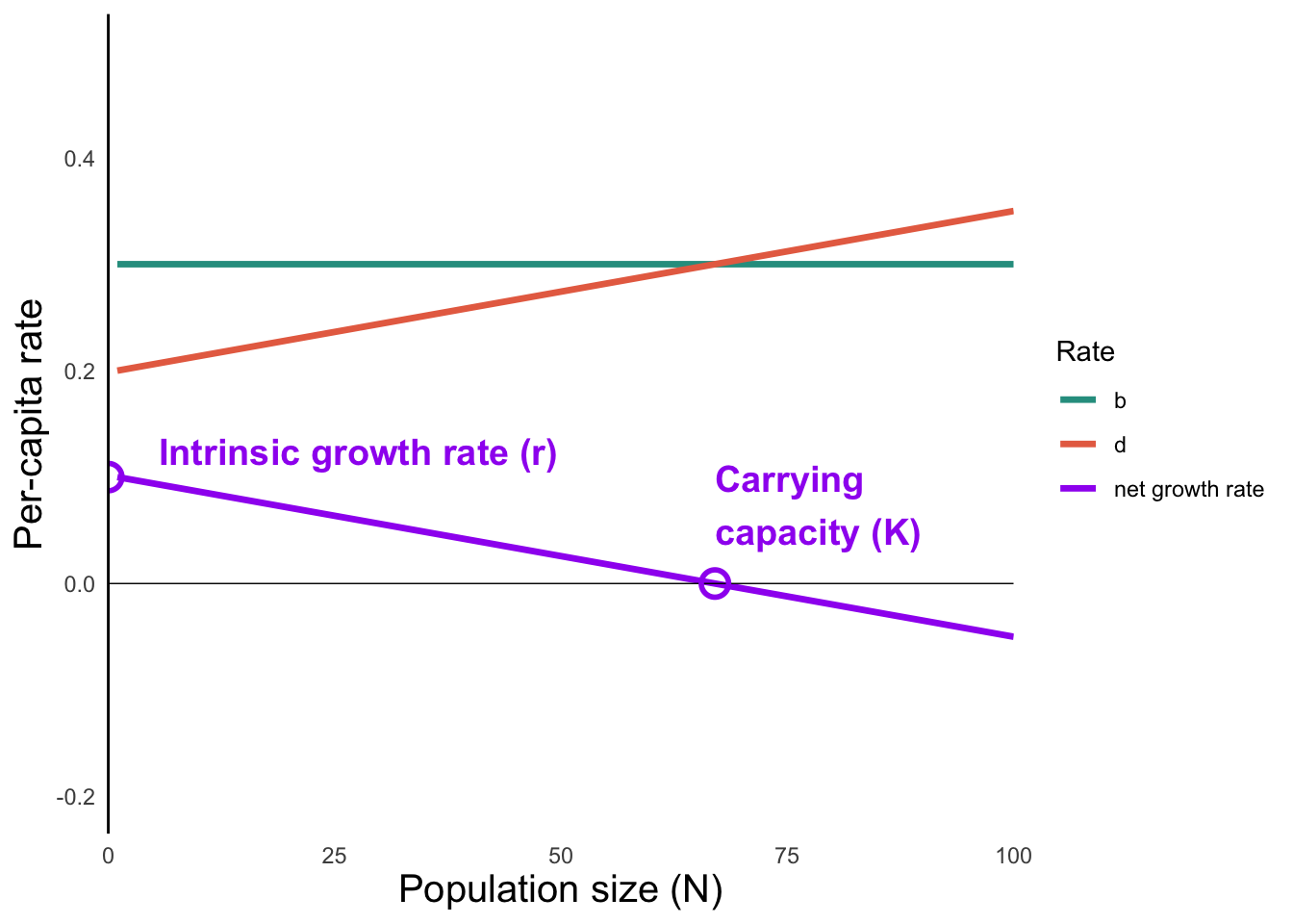
- Recall from algebra that we can use the “point-slope” approach for the slope of a line (\(y-y_1 = m(x - x_1)\))
- We know two points: \((0,r)\) and \((K,0)\)
- The slope of the line turns out to be \(-\frac{r}{K}\), which we write as \(\alpha\)
- And \(y\) gives the per-capita population growth rate \(\frac{1}{N}\frac{dN}{dt}\)
Population growth over time
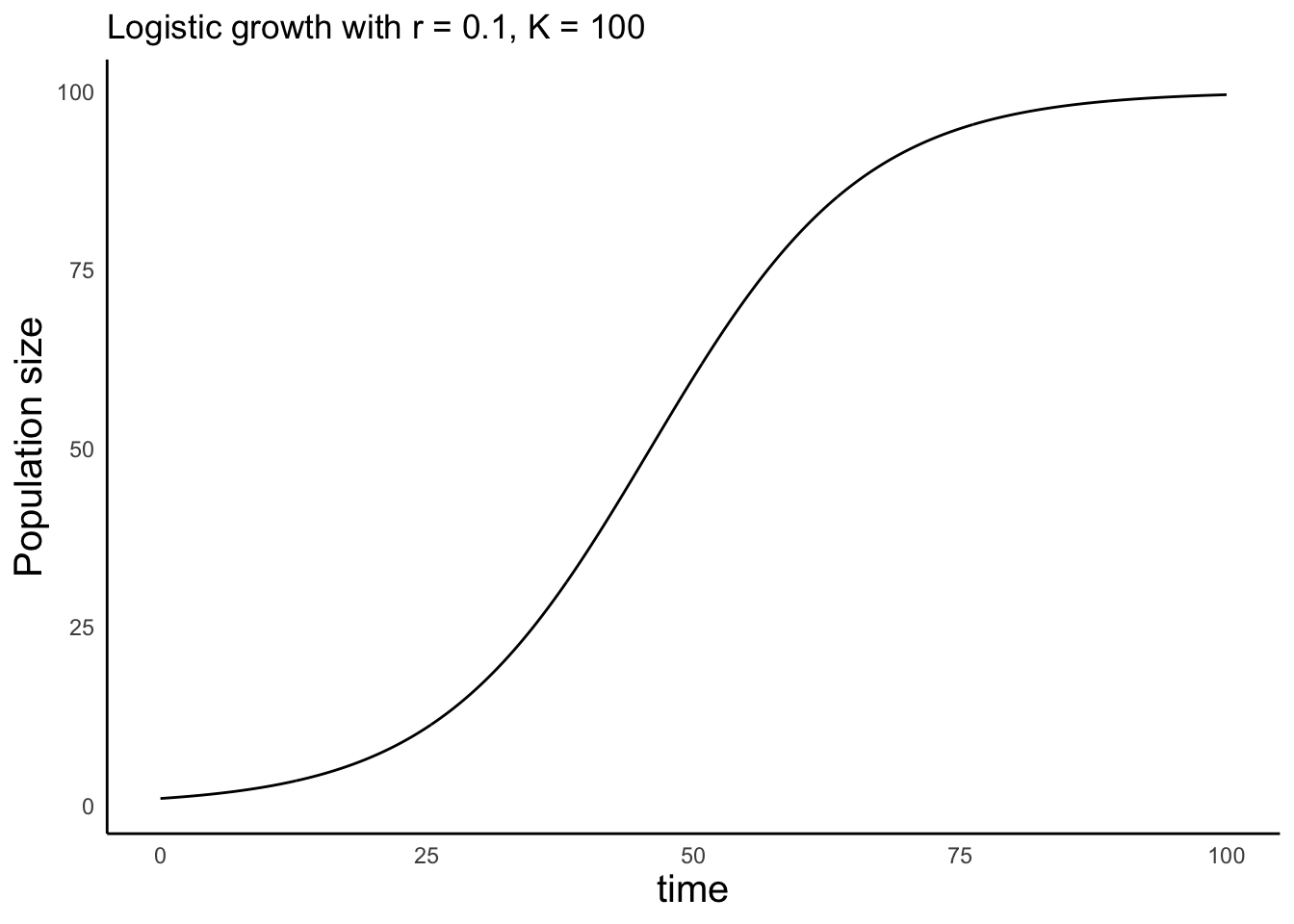
Population growth over time
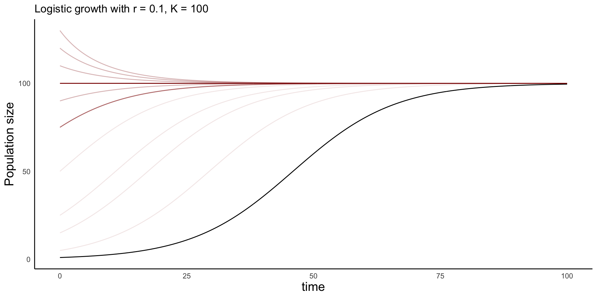
The population will converge to the carrying capacity no matter the initial size