Stability and Allee effects

Summary of logistic growth

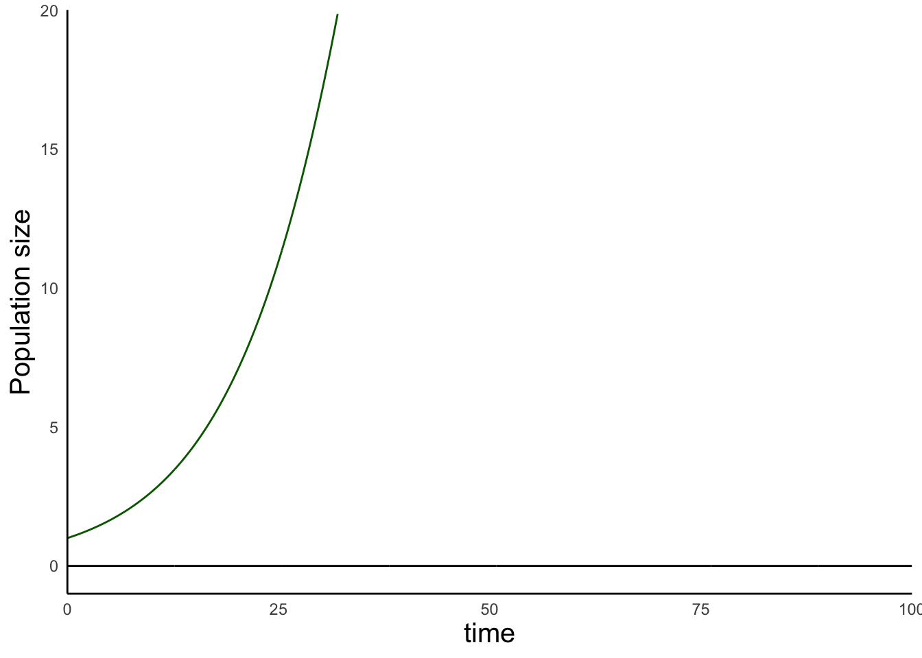
  • The exponential growth model predicts unbounded population growth (no equlibrium)
  • The logistic growth model relaxes one assumption (birth/death rates that change with \(N\))
  • Now allows population sizes to saturate at a carrying capacity
    • Biological realism, but also more parameters to estimate

Density-dependence in models

Exponential growth

\[\frac{dN}{dt} = rN\]

Logistic growth growth

\[\frac{dN}{dt} = rN\bigg(1-\frac{N}{K}\bigg)\]

Density-dependence in models

Exponential growth

\[\frac{dN}{dt} = rN\]

\[\frac{1}{N}\frac{dN}{dt} = r\]

Logistic growth growth

\[\frac{dN}{dt} = rN\bigg(1-\frac{N}{K}\bigg)\]

\[\frac{1}{N}\frac{dN}{dt} = r\bigg(1-\frac{N}{K}\bigg)\]

Summary of logistic growth

\[\frac{dN}{dt} = rN \bigg(1-\frac{N}{K}\bigg)\]

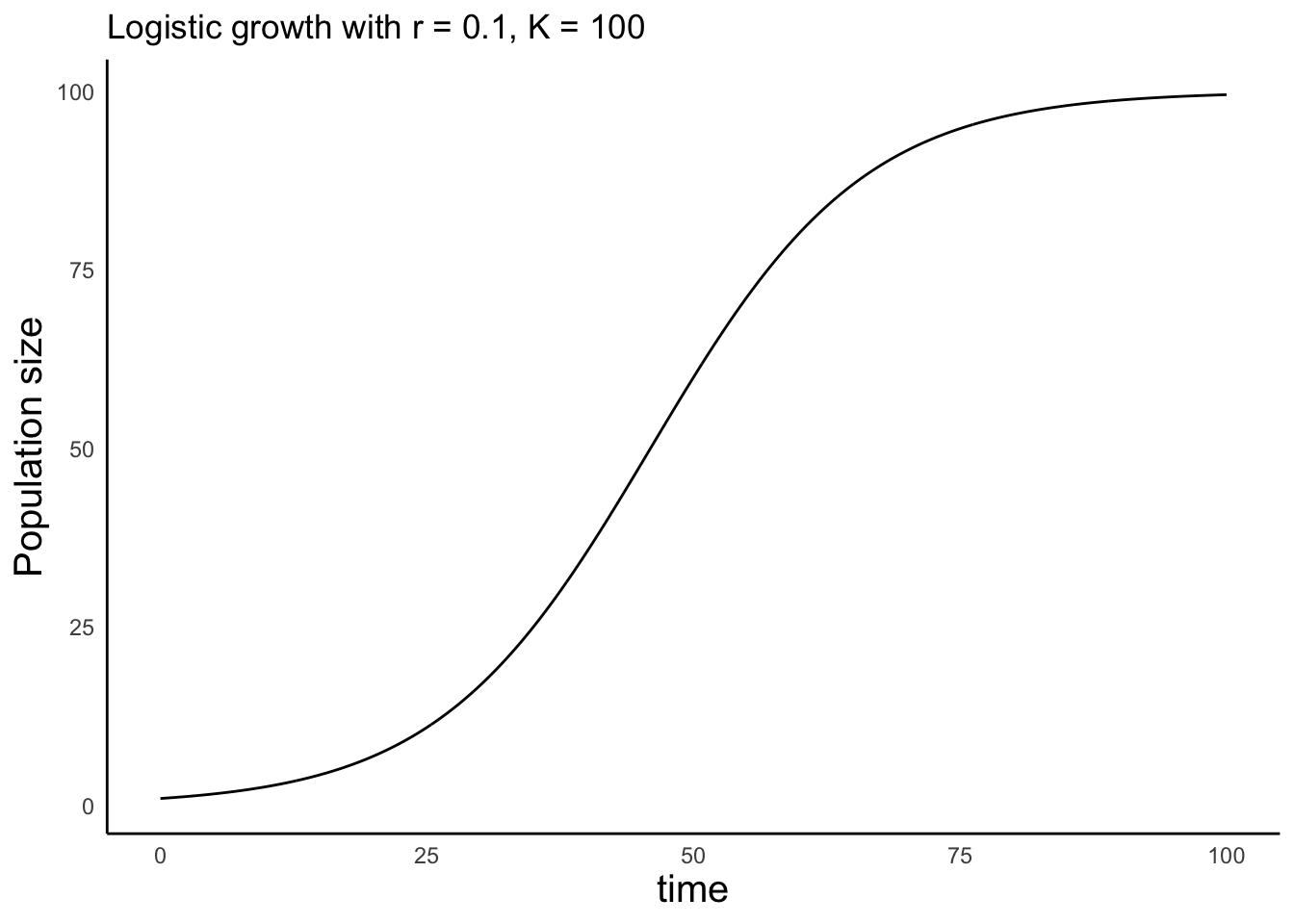
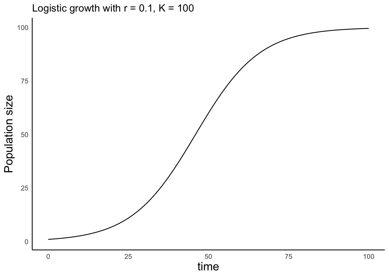
  • When population size is very small (\(N \to 0\)), \(\frac{N}{K} \to 0\), and the population grows ‘exponentially’
  • When population size is close to carrying capacity (\(N \to K\)), \(\frac{N}{K} \to 1\), and the population remains constant
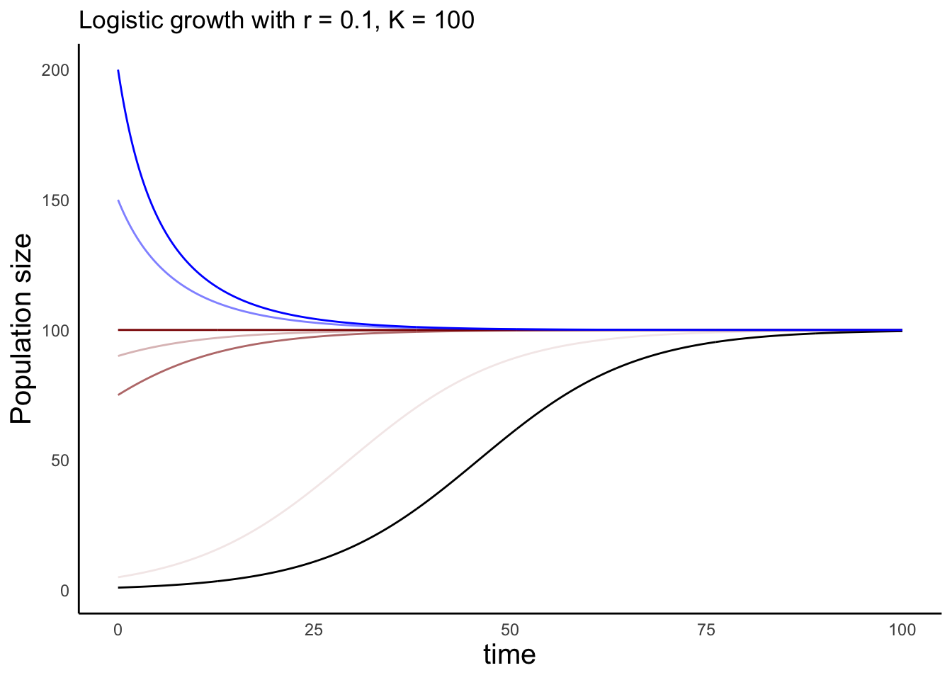
  • When population size exceeds carrying capacity (\(N > K\)), \(\frac{N}{K} > 1\), and the population growth rate is negative (shrinks)

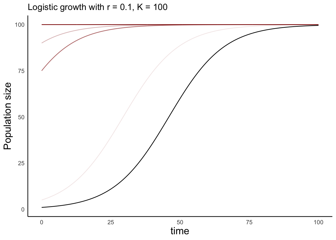
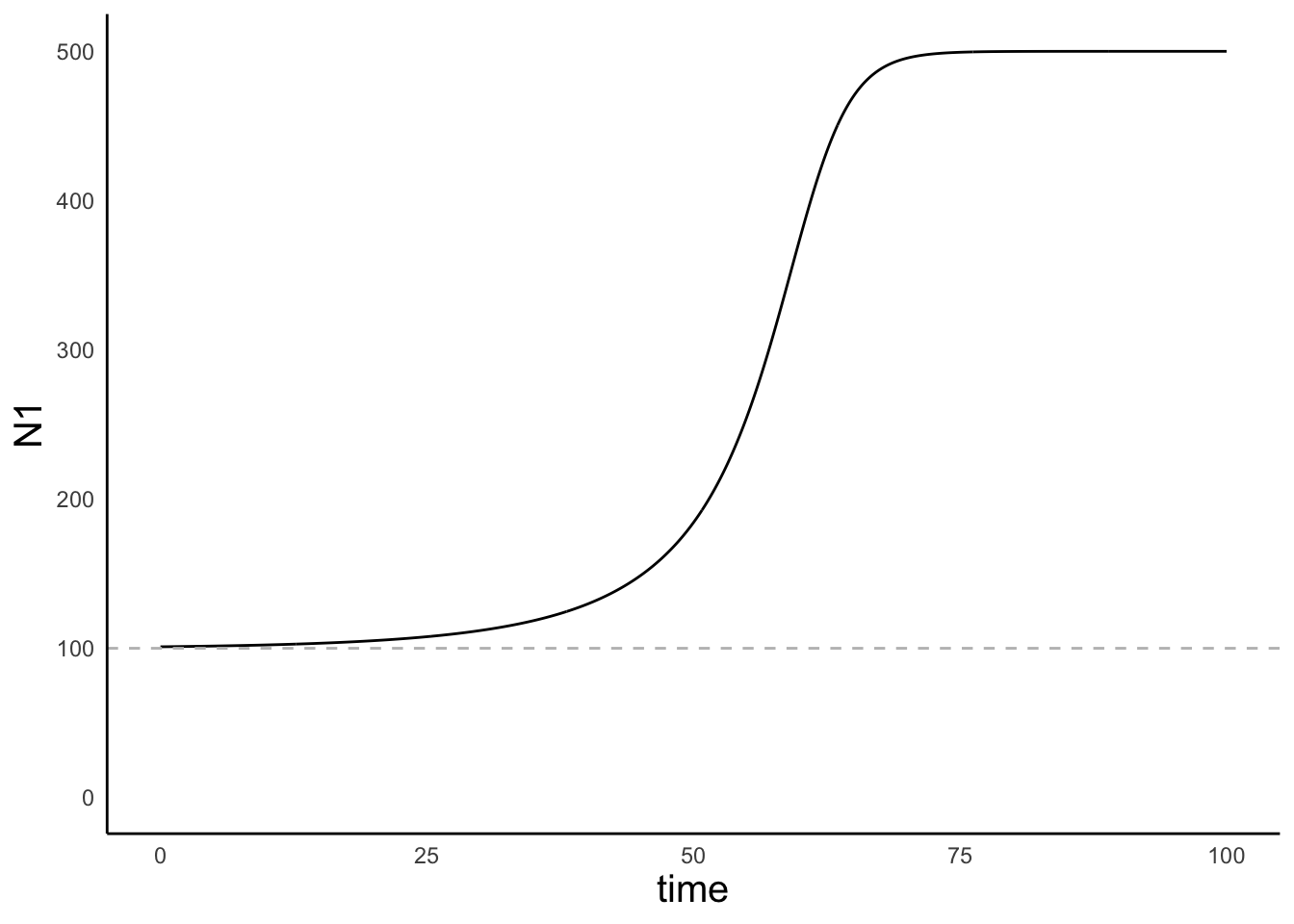
Population growth over time

What is the “equilibrium” of this system

  • Intuitively, we might say that the system is at equilibrium when it is at carrying capacity (\(K\))

  • What is special about this?

\[\frac{dN}{dt} = rN\bigg(1-\frac{K}{N}\bigg)\] When \(N = K\), \(\frac{dN}{dt} \to 0\).

This gets us back to the definition of equilibrium in ecological systems: no net change in the system (\(\frac{dN}{dt} = 0\))

But, what about other equilibria?

\[\boxed{\frac{dN}{dt} = rN\bigg(1-\frac{K}{N}\bigg) = 0} \text{ also happens when } N = 0\]

Thus, this system has two equilibrium points:

\[N = 0 \text{ and } N = K\]

Evaluating the stability of equilibrium points

  • Just because a system is “at equilibrium” doesn’t mean it will never change

  • The dynamics depend on the stability of the equilibrium

  • An equilibrium is considered (locally) stable if small perturbations cause the population to return to its original state.

  • Alternatively, an equilibrium is unstable if small perturbations cause the system to move away from the original state

Consider a population that is at equilibrium because \(N = 0\)

A small perturbation causes \(N = 1\) (e.g. an immigration event)

This means the equilibrium \(N = 0\) is an unstable equilibrium

Consider a population that is at equilibrium because \(N = K\)

A small perturbation causes \(N\) to shift slightly lower than \(K\) (e.g. a hurricane that kills a fraction of the individuals)

Alternatively, a small perturbation causes \(N\) to shift slightly higher than \(K\) (e.g. humans release additional individuals into the system)

Stability of the logistic equlibrium

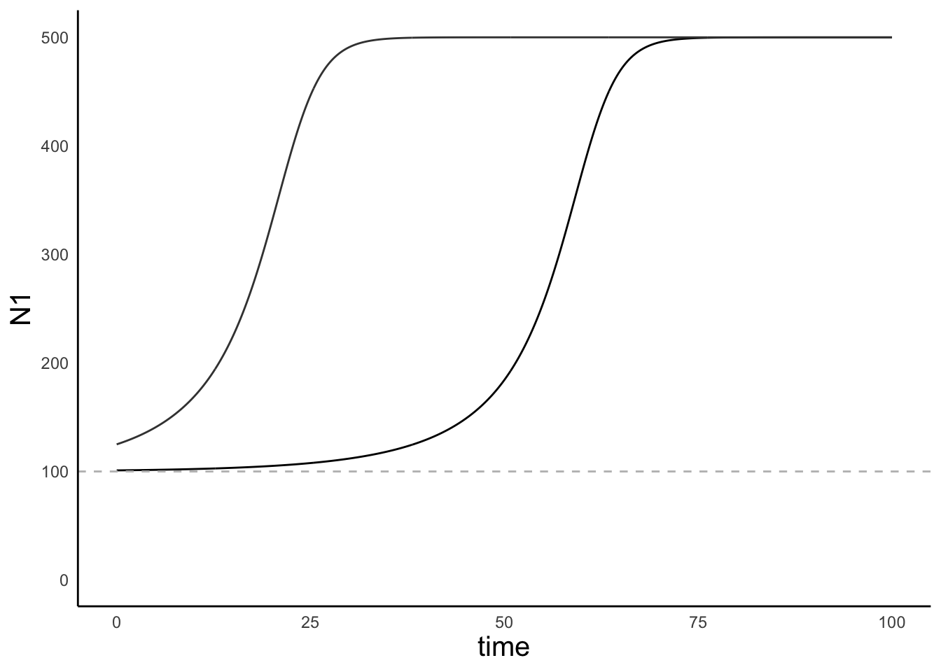
  • The past few slides show that the initial conditions (\(N\) at \(t=0\)) doesn’t change the equilibrium condition of the system
  • This makes it a Stable equilibrium
    • The system is robust to small perturbations

Evaluating assumptions Logistic Growth

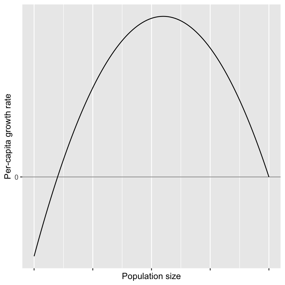
One of the implicit assumptions in the logistic growth model is that higher population density always results in reduced per-capita performance

We have discussed many reasons why this may not be true

Incorporate facilitation into logistic growth

  • Per-capita growth rate can increase with population size
  • Until some threshold, after which it declines again

Density-dependence with Allee effect

Incorporate facilitation into logistic growth

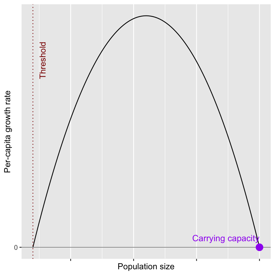
\[\frac{dN}{dt} = - rN \bigg( 1-\frac{N}{T} \bigg) \bigg( 1-\frac{N}{K} \bigg)\]

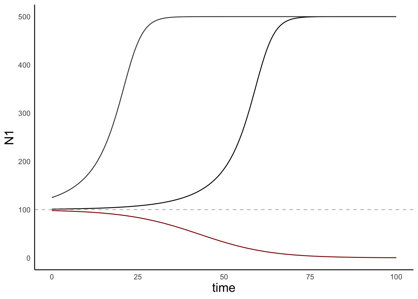
\(T\) is a threshold value – when populations are below this, fitness increases with population size

  • e.g. There might be a “Threshold” size of a wolf pack
  • below this threshold, it is hard to hunt, such that the population crashes to extinction
  • above this threshold, the population grows to carrying capacity

Equilibria and stability

\[\frac{dN}{dt} = - rN \bigg( 1-\frac{N}{T} \bigg) \bigg( 1-\frac{N}{K} \bigg)\]

This model has three equilibrium points:

\(N = 0\), \(N = T\), and \(N = K\)

Lessons from a model with facilitation

Lessons from a model with facilitation

Lessons from a model with facilitation

Equilibria and stability

\[\frac{dN}{dt} = - rN \bigg( 1-\frac{N}{T} \bigg) \bigg( 1-\frac{N}{K} \bigg)\]

This model has three equilibrium points:

\(N = 0\), \(N = T\), and \(N = K\)

What do we expect in terms of the stability for each of these equilibrium points?

\(N = 0 \to \text{stable equilibrium}\), \(N = T \to \text{unstable equilibrium}\), \(N = K \to \text{stable equilibrium}\)

Equilibria and stability

\[\frac{dN}{dt} = - rN \bigg( 1-\frac{N}{T} \bigg) \bigg( 1-\frac{N}{K} \bigg)\]

This model has three equilibrium points:

\(N = 0\), \(N = T\), and \(N = K\)

What do we expect in terms of the stability for each of these equilibrium points?

\(\boxed{N = 0 \to \text{stable equilibrium}}\), \(N = T \to \text{unstable equilibrium}\), \(N = K \to \text{stable equilibrium}\)

Density-dependence summary

  • Birth and death rates can depend on the size of the population
  • When this happens, the population growth rate will also change with population size
  • Population growth rate declines linearly with \(N\) in the logistic model
    • This gives rise to a very stable equilibrium…
    • … but it isn’t realistic in all cases
  • When we account for Allee effects (birth rates grow or death rates decline with bigger populations, i.e. positive density-dependence), we encounter unstable equilibria
    • Populations falling below the “threshold” crash to extinction