A simple model of two-species competition, pt. 2

Last time

Why focus on competition?

• Last time, I mentioned the historical basis
• There is also the puzzle that ecologists have been intrigued by: if there are multiple species that “behave” the same way, how can they persist? Why does one not go extinct?
  • Note that here, “behave” has a broad definition: How does the organism respond to and change the environment?

We will use the logistic growth model as a starting point to think about competition between two species.

• Remember that logistic growth can be conceptually thought of as “competition within just 1 species”
• It is this within-species competition that sets an upper value for a equilibrium population size, AKA carrying capacity

\[\frac{dN_1}{dt} = r_1N_1(1-\alpha_{11}{N_1})\]

\[\frac{dN_1}{dt} = r_1N_1(1-\alpha_{11}{N_1})\]

• \(\alpha_{11}\) is the strength of within-population competition (also called intraspecific competition)

• When there is competition between species, the growth rate of species 1 (\(\frac{dN_1}{dt}\)) is also affected by species 2

\[\frac{dN_1}{dt} = r_1N_1(1-\alpha_{11}{N_1} - \text{competition from species 2})\]

Similarly, the growth rate of Species 2 is limited by intraspecific and interspecific competition

\[\frac{dN_2}{dt} = r_2N_2(1-\alpha_{22}{N_2} - \text{competition from species 1})\]

\[\frac{dN_1}{dt} = r_2N_1(1-\alpha_{11}{N_1} - \text{competition from species 2})\]

If we define \(\alpha_{12}\) as the competitive impact of Species 2 on Species 1, then we can formalize how competition manifests:

\[\frac{dN_1}{dt} = r_1N_1(1-\alpha_{11}{N_1} - \alpha_{12}N_2)\]

Similarly for Species 2:

\[\frac{dN_2}{dt} = r_2N_2(1-\alpha_{22}{N_2} - \alpha_{21}N_1)\]

A simple model of pairwise competition

\[\frac{dN_1}{dt} = r_1N_1(1-\alpha_{11}{N_1} - \alpha_{12}N_2)\]

\[\frac{dN_2}{dt} = r_2N_2(1-\alpha_{22}{N_2} - \alpha_{21}N_1)\]

Just as in the past, we can evaluate:

• What are the equilibrium points?
• What is the stability of these equilibrium points?

Why evaluate equilibria?

• If we are interested in how biodiversity persists (i.e. how do two very similar species coexist), then we can express this question formally:

  • What has to be true for multiple species to persist at equilibrium?
  • Under what conditions is the persistence of biodiversity a stable condition?

Let’s try to understand the model

\[\frac{dN_1}{dt} = r_1N_1(1-\alpha_{11}{N_1} - \alpha_{12}N_2)\]

\[\frac{dN_2}{dt} = r_2N_2(1-\alpha_{22}{N_2} - \alpha_{21}N_1)\]

What determines the strength of competition?

The size of \(\alpha\) reflects “how competitive” interactions are:

• Strong competition (high \(\alpha\)) happens when each additional individual of a species strongly reduces fitness of other individuals

• In other words, \(\alpha_{ij}\) are determined the degree to which an individual of species \(j\) changes the environment in a way that suppresses individuals of species \(i\)

  • If species 1 competes strongly with itself, high \(\alpha_{11}\)
  • If species 1 competes strongly with species 2, high \(\alpha{21}\)

What makes intra-specific competition different from inter-specific competition?

Why are \(\alpha_{ii}\) and \(\alpha_{ij}\) different from one another?

• When the species have highly overlapping niches, intra-specific and inter-specific \(\alpha\)s are very similar: \(\alpha_{ii} \approx \alpha_{ij}\)

• When two species have highly distinct niches, intra-specific competition is very low: \(\alpha_{ij} \approx 0\)

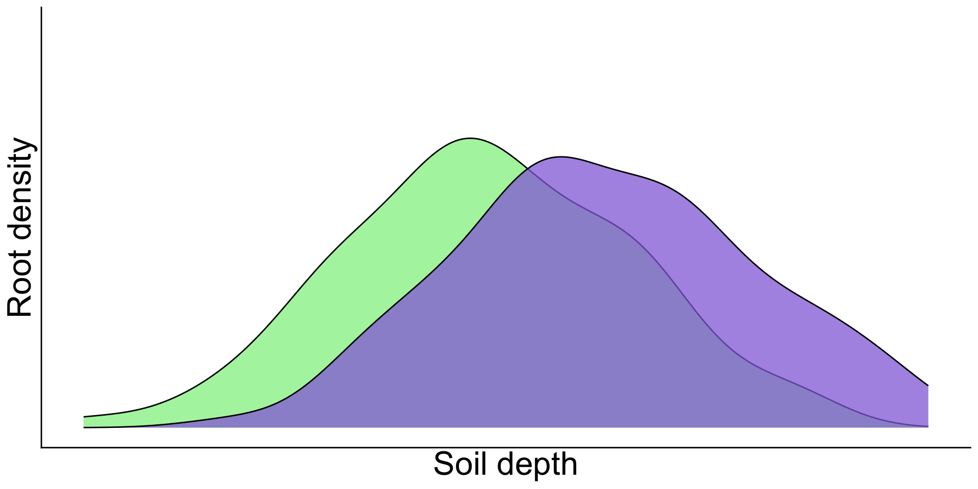
e.g. if two plant species get water from the same depth in the soil, liklihood of high interspecific competition

• High \(\alpha_{12}\) and \(\alpha{21}\) expected

Whereas if two species get water from distinct parts of the soil profile, lower competition between the two species

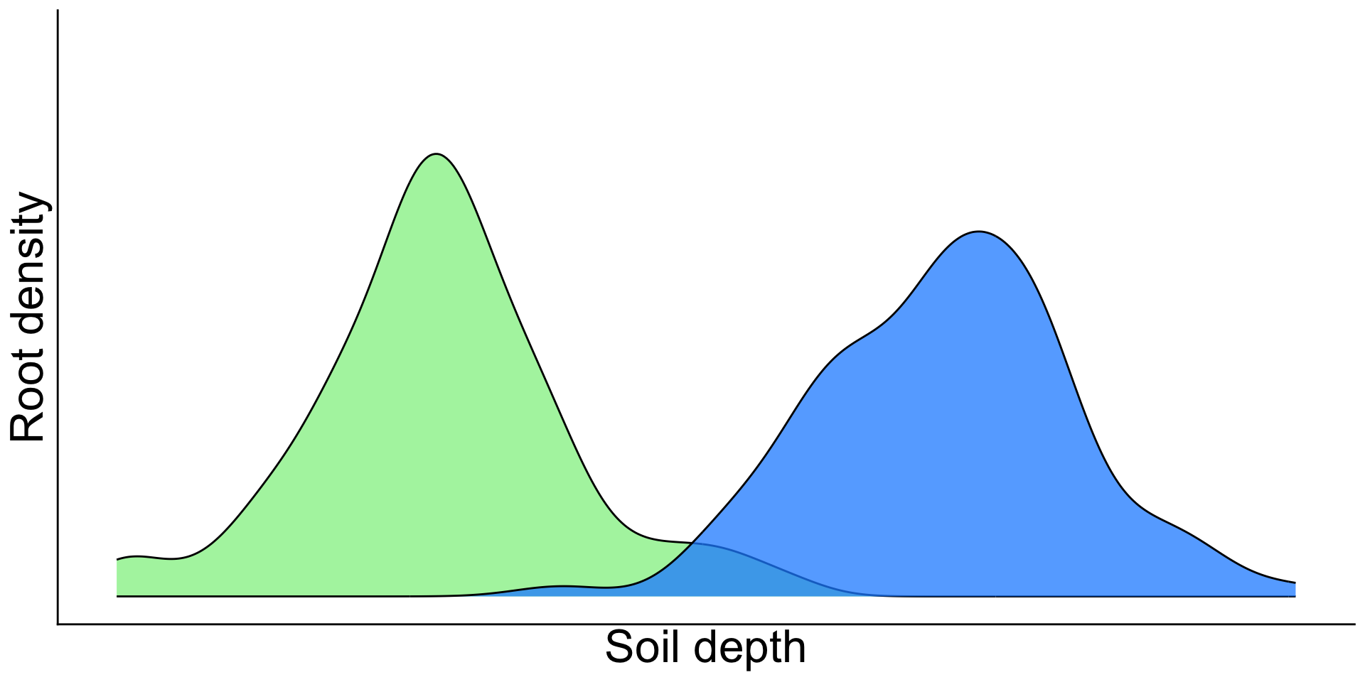
• Low \(\alpha_{12}\) and \(\alpha{21}\) expected

What are the equilibrium conditions of the model?

\[\frac{dN_1}{dt} = r_1N_1(1-\alpha_{11}N_1 - \alpha_{12}N_2)\]

\[\frac{dN_2}{dt} = r_2N_2(1-\alpha_{21}N_1 - \alpha_{22}N_2)\]

• Have to solve this as a system of equations (What are combinations of \(N_1\) and \(N_2\) that yield equilibrium?)
  • We will solve for \(\frac{dN_1}{dt} = 0\) and then \(\frac{dN_2}{dt} = 0\)

• Let’s consider two “extreme” cases:
  • Extreme case 1: Can the system be at equilibrium if Species 1 is growing alone (no species 2 present)?
  • We will call this a “single-species equilibrium”

Single-species equilibrium for Species 1

• If species 1 is growing alone, the equation simplifies:

\[\frac{dN_1}{dt} = r_1N_1(1-\alpha_{11}N_1 - \boxed{\alpha_{12}N_2})\]

• If the term in the box goes to zero, the equation simplifies to the logistic growth model for species 1!

• This gives us the first equilibrium point: \(\big(N_1 = \frac{1}{\alpha_{11}}, N_2 = 0\big)\)

Single-species equilibrium for Species 1

• Alternatively, \(\frac{dN_1}{dt} = 0\) can happen if \(N_1=0\) but \(N_2\) is very high.

\[\frac{dN_1}{dt} = r_1N_1(1-\boxed{\alpha_{11}N_1} - {\alpha_{12}N_2})\]

• If the term in the box goes to zero, the equation simplifies to the logistic growth model for species 2!
• If we solve this for \(\frac{dN_1}{dt} = 0\), we see that equilibrium is also possible if \(\big(N_1 = 0, N_2 = \frac{1}{\alpha_{12}}\big)\)
• This is the second equilibrium point.

Visualizing Species 1’s equilibria

• Recall two equilibrium points:
  • \(\big(N_1 = \frac{1}{\alpha_{11}}, N_2 = 0\big)\)
  • \(\big(N_1 = 0, N_2 = \frac{1}{\alpha_{12}}\big)\)
• If we want to visualize these, we need a graph in two dimensions

How to add \(\big(N_1 = \frac{1}{\alpha_{11}}, N_2 = 0\big)\) and \(\big(N_1 = 0, N_2 = \frac{1}{\alpha_{12}}\big)\) to a plot?

• \(N_1\) and \(N_2\) need to be the two axes of the plot.

How to add \(\big(N_1 = \frac{1}{\alpha_{11}}, N_2 = 0\big)\) and \(\big(N_1 = 0, N_2 = \frac{1}{\alpha_{12}}\big)\) to a plot?

• \(N_1\) and \(N_2\) need to be the two axes of the plot.

Single-species equilibrium for Species 2

\[\frac{dN_2}{dt} = r_2N_2(1-\alpha_{22}N_2 - \boxed{\alpha_{21}N_1})\]

• In fact, if the boxed term goes to zero, the equation simplifies to the logistic growth model for species 2!

• This gives us the second equilibrium point: \(\big(N_1 = 0, N_2 = \frac{1}{\alpha_{22}} \big)\)

Single-species equilibrium for Species 2

\[\frac{dN_2}{dt} = r_2N_2(1-\boxed{\alpha_{22}N_2} - \alpha_{21}N_1)\]

• Alternatively, there can be zero individuals of Species 2 and many of species 1 (boxed term goes to zero)

• This gives us the second equilibrium point: \(\big(N_1 = \frac{1}{\alpha_{21}}, N_2 = 0 \big)\)

Plotting Species 2’s single-species equilibrium points

Species 2’s single-species equilibria are:

\(\big(N_1 = 0, N_2 = \frac{1}{\alpha_{22}} \big)\) and \(\big(N_1 = \frac{1}{\alpha_{21}}, N_2 = 0 \big)\)