A simple model of two-species competition

Approach to modeling competition

We already saw the effects of competition within a species: population growth slows down as the population gets big
Logistic growth dynamics consider a species whose individuals compete with each other

\[\frac{dN_1}{dt} = r_1N_1(1-\frac{N_1}{K_1})\]

Rewrite on a per-capita basis

\[\frac{1}{N_1}\frac{dN_1}{dt} = r_1(1-\frac{N_1}{K_1})\]

Redefine \(K_1 = \frac{1}{\alpha_{11}}\)

\[\frac{1}{N_1}\frac{dN_1}{dt} = r_1(1-\alpha_{11}{N_1})\]

Where \(\alpha_{11}\) is the strength of competition within species.

We can now think extend this logic to a second species

Two-species competition

\[\frac{1}{N_1}\frac{dN_1}{dt} = \overbrace{r_1}^{\substack{\text{growth}\\\text{without}\\ \text{competition}}} \overbrace{(1-\alpha_{11}{N_1})}^{\substack{\text{reduction due}\\ \text{to competition}}}\]

\(\alpha_{11}\) is the strength of competition within species,
\(\alpha_{12}\) is the impact of species \(2\) on species \(1\).

\[\frac{1}{N_1}\frac{dN_1}{dT} = r_1(1-\alpha_{11}N_1 - \alpha_{12}N_2)\]

\[\frac{1}{N_2}\frac{dN_2}{dT} = r_2(1-\alpha_{21}N_1 - \alpha_{22}N_2)\]

\(\alpha_{22}\) is the strength of competition within species,
\(\alpha_{21}\) is the impact of species \(1\) on species \(2\).

Let’s dig into how the model works.

\[\frac{1}{N_1}\frac{dN_1}{dT} = r_1(1-\alpha_{11}N_1 - \alpha_{12}N_2)\]

What happens if species 1 is growing alone?

\[\frac{1}{N_1}\frac{dN_1}{dT} = r_1(1-\alpha_{11}N_1)\]

Growth to Species 1’s carrying capacity (\(N_1^* = \frac{1}{\alpha_{11}} = K_1\))

Similarly, if Species 2 is growing alone, it will grow to its carrying capacity \(N_2^* = \frac{1}{\alpha_{22}} = K_2\)

But what happens if both species are present in the system?

Possible outcomes of two species competing:

Both species can have stable coexistence
Species 1 can win, and exclude Species 2
Species 2 can win, and exclude Species 1
“It depends” – whichever species comes first, wins in competition.

How to predict the outcome for any given pair of species?

What conditions enable coexistence?

Defining species coexistence

As ecologists, we are not just interested in whether it is possible to see two species in the same place at the same time.
We want to know whether species can coexist at equilibrium, and whether this equlibrium is stable.

Signature of stable coexistence:

System is at equilibrium (\(\frac{dN_1}{dt} = 0\) and \(\frac{dN_2}{dt} = 0\))
Both species are present (abundance > 0)
If the system is pushed a bit away from equilibrium, it will return to the same equilibrium

Under what conditions do both species co-exist?

Approach: Graphical analysis of the competition model

New type of visualization: phase space (AKA “state space”)
New type of analysis: null-cline analysis
(AKA “zero net-growth isocline”)

We have already seen a phase space model

Now, the challenge is to extend this to two dimensions.
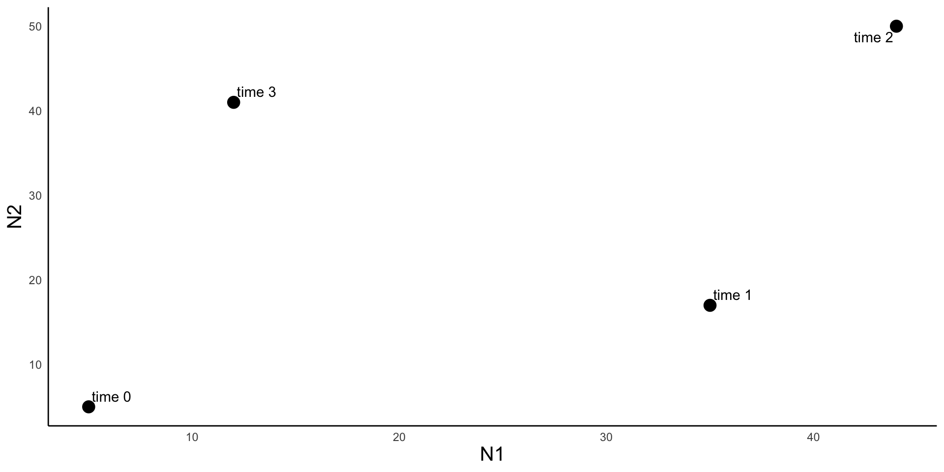
Instead of a number line (1-dimension), we need a graph with an X- and a Y-axis (2-dimensional)
The number line represented the abundance of our species; now each axis represents the abundance of one of our two species
- X-axis is abundance of species 1, Y-axis is abundance of species 2
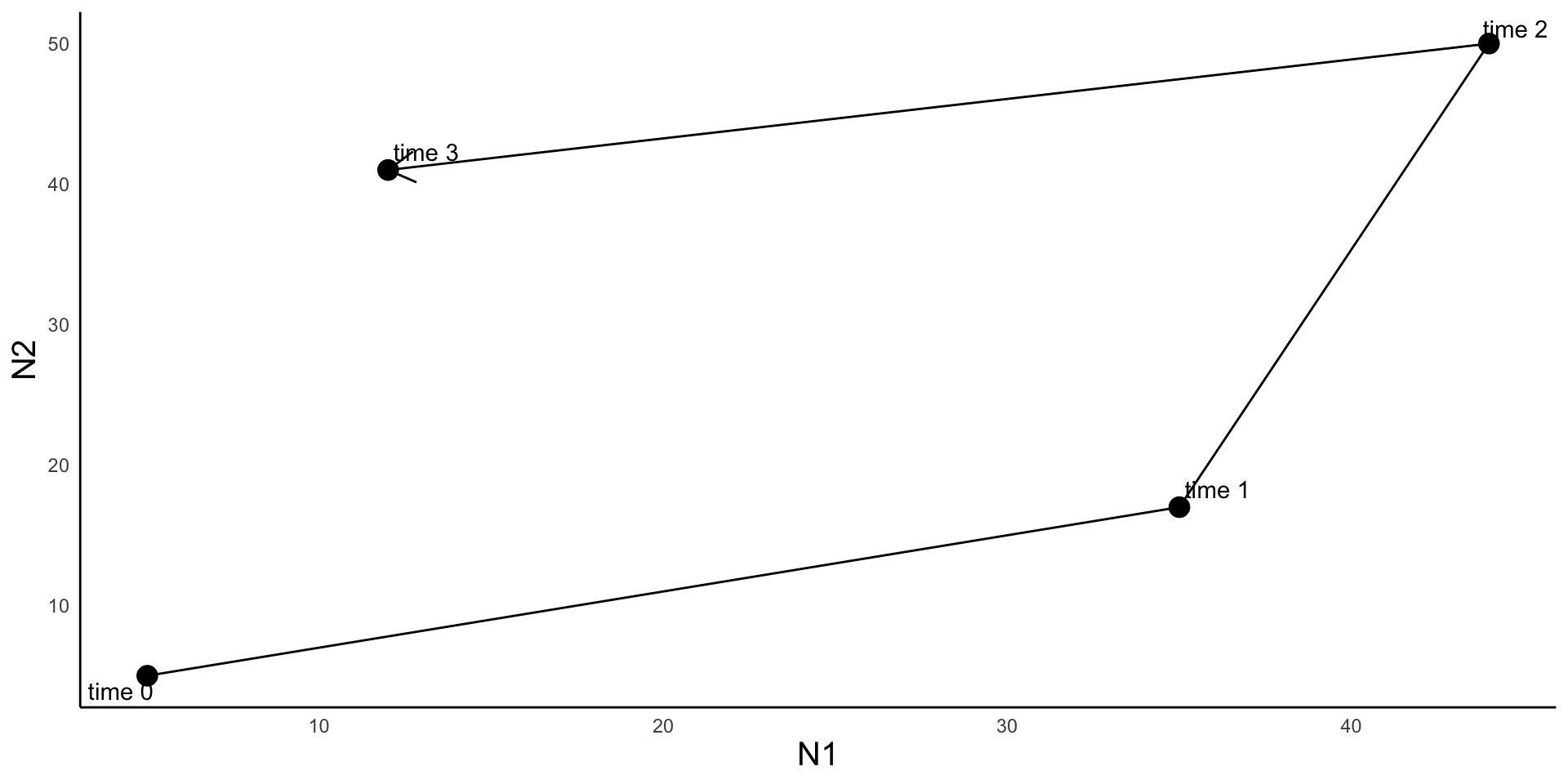
Any point on the graph represents a possible state of the system
Lines on the graph show how a system changes through time (trajectory)

Null-cline analyses (AKA zero net growth isocline analysis)

Is there any point in this space that allows the system to not change over time? (i.e. to reach equilibrium)
We can approach this problem one axis at a time.
Key questions:
- At what points does the abundance of species 1 (\(N_1\)) not change?
- At what points does the abundance of species 2 (\(N_2\)) not change?

At what points does the abundance of species 1 (N1) not change?

\[\frac{dN_1}{dT} = r_1N_1(1-\alpha_{11}N_1 - \alpha_{12}N_2)\]

Two “extreme” cases…

When species 1 is at its carrying capacity, and species 2 is not around
- \(N_1 = \frac{1}{\alpha_{11}}, N_2 = 0\)
When there are so many individuals of Species 2 that Species 1 cannot begin to grow
- When does that happen?
- \(N_1\) is low (0), and \(N_2\) is… some high number

\[\frac{1}{N_1}\frac{dN_1}{dT} = r_1(1-\alpha_{11}N_1 - \alpha_{12}N_2)\]

Solve for \(\frac{dN_1}{dT} = 0, N_1 = 0, N_2 > 0\) (on paper)

At what points does the abundance of species 1 (N1) not change?

When species 2 is absent, and species 1 is at its carrying capacity
- \(N_2 = 0, N_1 = \frac{1}{\alpha_{11}}\)
When there are so many individuals of Species 2 that Species 1 cannot begin to grow
- When does that happen?

\(N_1 = 0, N_2 = \frac{1}{\alpha_{12}}\)

Summary of the null-cline analysis so far:

We set out to find cases where \(N_1\) doesn’t change, i.e. \(dN_1/dt = 0\)
We identified two extreme scenarios:
- \(N_1 = 1/\alpha_{11}, N_2 = 0\)
- \(N_1 = 0, N_2 = 1/\alpha_{12}\)
We can put these two extreme points on the state space graph.

Draw state space with Species 1 equilibrium points (on paper)

Growth of species 1 is also zero for intermediate combinations between these extremes

These intermediate combinations are defined by the line connecting the two extremes.
We can solve for the equation of this line.

\[\frac{1}{N_1}\frac{dN_1}{dT} = r_1(1-\alpha_{11}N_1 - \alpha_{12}N_2)\]

\[N_2^* = \frac{1-\alpha_{11}N1}{\alpha_{12}} \]

\[N_2^* = \frac{1-\alpha_{11}N1}{\alpha_{12}} = \frac{1}{\alpha_{12}} + \frac{\alpha_{11}}{\alpha_{12}}N_1\]

Growth of species 1 is also zero for intermediate combinations between these extremes

\[\frac{dN_1}{dT} = r_1N_1(1-\alpha_{11}N_1 - \alpha_{12}N_2)\]

\[N_2^* = \overbrace{\frac{1}{\alpha_{12}}}^{\text{y-intercept}} - \overbrace{\frac{\alpha_{11}}{\alpha_{12}}}^{\text{slope}}N_1\]

This is the equation of the null-cline for species 1 (AKA zero net-growth isocline, or ZNGI)

Draw state space with Species 1 equilibrium points, plus intermediate line (on paper)

Discussion point: What happens on either side of the null-cline?

Recall the key questions of null-cline analysis:

Key questions:
At what points does the abundance of species 1 (\(N_1\)) not change?
- \(N_1 = 1/\alpha_{11}, N_2 = 0\);
  \(N_1 = 0, N_2 = 1/\alpha_{12}\);
  \(N_2 = \frac{1}{\alpha_{12}} - \frac{\alpha_{11}}{\alpha_{12}}N_1\)

At what points does the abundance of species 2 (\(N_2\)) not change?

At what points does the abundance of species 2 (\(N_2\)) not change?

When species 1 is not around, and species 2 is at its carrying capacity
- \(N_1 = 0, N_2 = 1/\alpha_{22}\)
When there are so many individuals of Species 1 that Species 2 cannot begin to grow
- \(N_1\) is some high number… and \(N_2\) is low (0)
- Following algebra, \(N_1 = 1/\alpha_{21}, N_2 = 0\)
We can add these two extremes to the state space plot

Growth of species 2 is also zero for intermediate combinations between these extremes

\[\frac{dN_2}{dT} = r_2N_2(1-\alpha_{21}N_1 - \alpha_{22}N_2)\]

\[N_2^* = \frac{1}{\alpha_{22}} - \frac{\alpha_{21}}{\alpha_{22}}N_1\]

This is the equation of the null-cline for species 2 (AKA zero net-growth isocline, or ZNGI)

Add null-cline to state space

What happens on either side of the nullcline?

Graphical analysis of the Lotka-Volterra competition model

Review:

Our goal is to identify conditions under which both species can coexist at equilibrium
Being ‘at equilibrium’ means \(dN_1/dt = dN_2/dt = 0\)
Null-cline analysis lets us find the conditions at which \(dN_1/dt = 0\), and the conditions at which \(dN_2/dt\)
There are a couple of ‘extreme’ cases (e.g. one species at carrying capacity, and the other absent), and a whole bunch of in-between cases that result in \(dN_1/dt = 0\) or \(dN_2/dt = 0\)

Test your recollection

Consider a pair of species that interact with the following strength:
- \(\alpha_{11} = 0.01\), \(\alpha_{12} = 0.005\), \(\alpha_{22} = 0.02\), \(\alpha_{21} = 0.001\)
- (\(\frac{1}{0.01} = 100,\ \frac{1}{0.01} = 200,\ \frac{1}{0.02} = 50,\ \frac{1}{0.001} = 1000\))
On separate graphs, draw the isoclines for species 1 and 2.