What are ways in which these reductionist approaches help us make sense of the whole?
General insight: more coexistence under stronger within-species limitation than between-species limitation
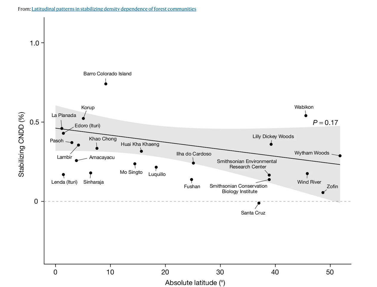
Is there more biodiversity in forests where within-species limitation is stronger?
Figure from Hulsman et al. 2024 in Nature, “Latitudinal patterns in stabilizing density dependence of forest communities”
General insight: Relative interaction strengths shape competitive outcomes
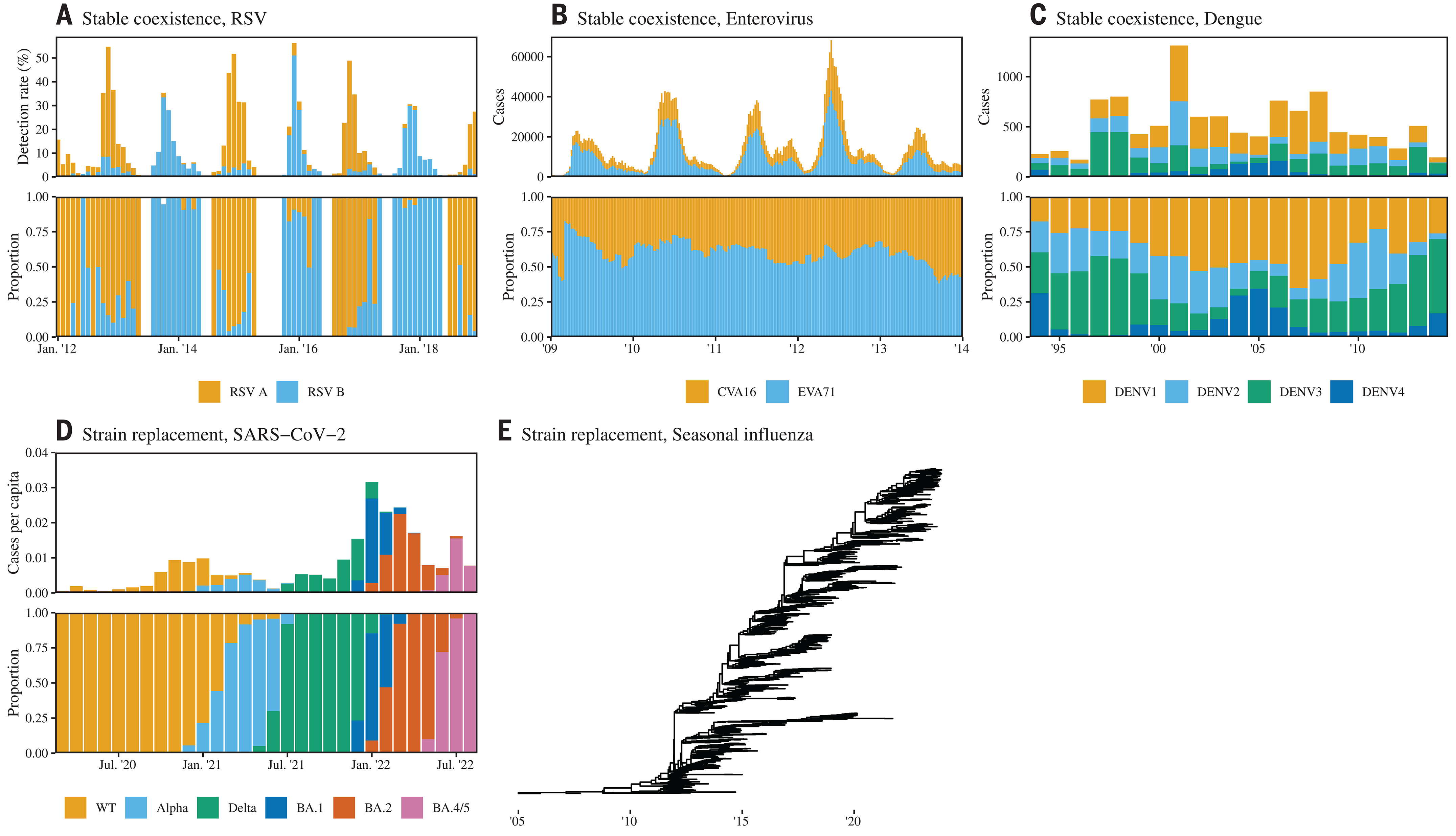
Can we understand pathogen co-infections based on coexistence theory?
Figure from Park et al. in Science, 2024, “Predicting pathogen mutual invasibility and co-circulation”
We address this gap by developing a pathogen invasion theory (PIT) based on modern ecological coexistence theory and testing the resulting framework against empirical systems. […] PIT unifies existing ideas about pathogen co-circulation, offering a quantitative framework for predicting the emergence of novel pathogen strains
In the previous unit, we explored how a reductionist approach can be applied to the study of species competition:
What can we learn from a similar approach to consumer–resource dynamics?
Building a simple consumer–resource system
Consider the dynamics of a “consumer” species \(C\) and a “resource” species \(R\)
The resource species has plenty of resources available and can grow exponentially…
… but it is suppressed by the consumer.
The consumer is a specialist (only eats the “resource” species)
(If there is no resource around, the consumer population dies out)
The consumer loses energy at some rate (maintenance cost)
How should the abundances of consumers and resources change over time? (\(\frac{dR}{dt}\) and \(\frac{dC}{dt}\))
Resource species dynamics
The resource species has plenty of resources available and can grow exponentially…
… but it is suppressed by the consumer.
\[\frac{dR}{dt} = \text{exponential growth - loss to consumer}\]
\[\frac{dR}{dt} = rR - aRC\]
\(R\) is the abundance of the resource species
\(r\) is the intrinsic growth rate of the resource
\(a\) is the attack rate of the consumer on the resource
\(C\) is the abundance of the consumer species
Consumer species dynamics
The consumer is a specialist (only eats the “resource” species)
The consumer loses energy at some rate (maintenance cost)
\[\frac{dC}{dt} = \text{growth from consumption - energy loss}\]
\[\frac{dC}{dt} = eaRC - mC\]
\(C\) is the abundance of the consumer species
\(a\) is the attack rate of the consumer on the resource
\(e\) is the efficiency with which consumer uses the energy it gets from resource
\(R\) is the abundance of the resource species
\(m\) is the maintenance cost of the consumer species
Lotka-Volterra consumer-resource system
\[\frac{dR}{dt} = rR - aRC\]
\[\frac{dC}{dt} = eaRC - mC\]
Some “obvious” takeaways:
If consumer species is absent (\(C = 0\)), the resource species grows exponentially
If the resource species is absent (\(R = 0\)), the consumer species dies out
Lotka-Volterra consumer-resource system
\[\frac{dR}{dt} = rR - aRC\]
\[\frac{dC}{dt} = eaRC - mC\]
Some more takeaways:
If the consumer attacks the resource at a very high rate (\(\uparrow a\)), resource populations will be suppressed, and consumer population grows more rapidly
If the consumer is very efficient at getting energy from the resource (\(\uparrow e\)), the consumer populations grow more rapidly
If consumer has high maintenance cost (\(\uparrow m\)), consumer populations will be suppressed
Equlibrium in C-R systems
Given the consumer–resource dynamics equations:
\[\frac{dR}{dt} = rR - aRC\]
\[\frac{dC}{dt} = eaRC - mC\]
Where does equilibrium occur?
How can we illustrate this in state-space?
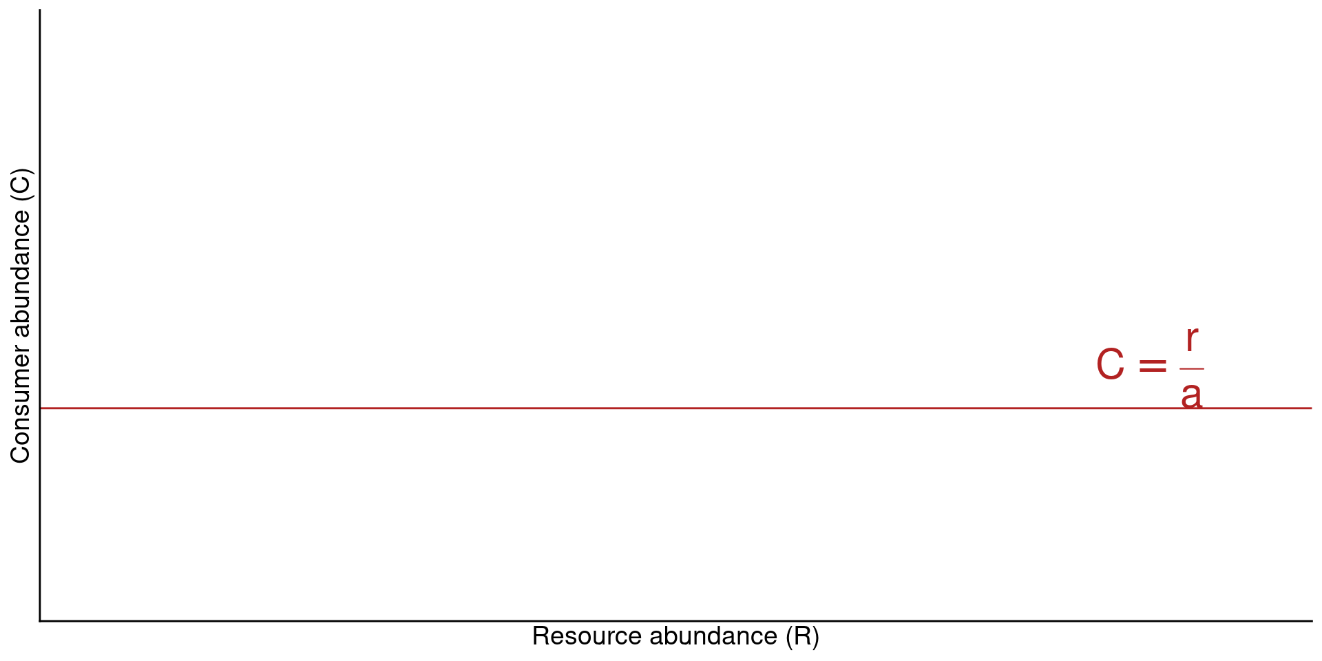
Equilibrium analysis of Resource
\[\frac{dR}{dt} = rR - aRC = 0\]
\[rR = aRC\]
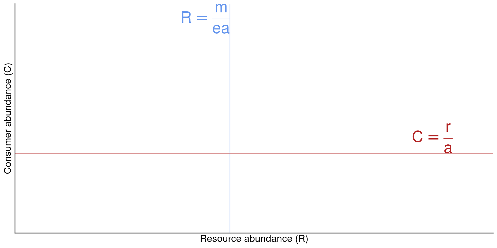
\[C^* = \frac{r}{a}\]
Interpretation: There is a set abundace of the consumer \(C\) that would cause the resource \(R\) to be at equilibrium.
If the resource grows slowly (low \(r\)), this happens at smaller abundances of the consumer
And/or if the consumer attacks the resource at a high rate (high \(a\)), this happens at smaller abundances of the consumer
Equlibrium analysis of consumer
\[\frac{dC}{dt} = eaRC - mC = 0\]
\[eaRC = mC\]
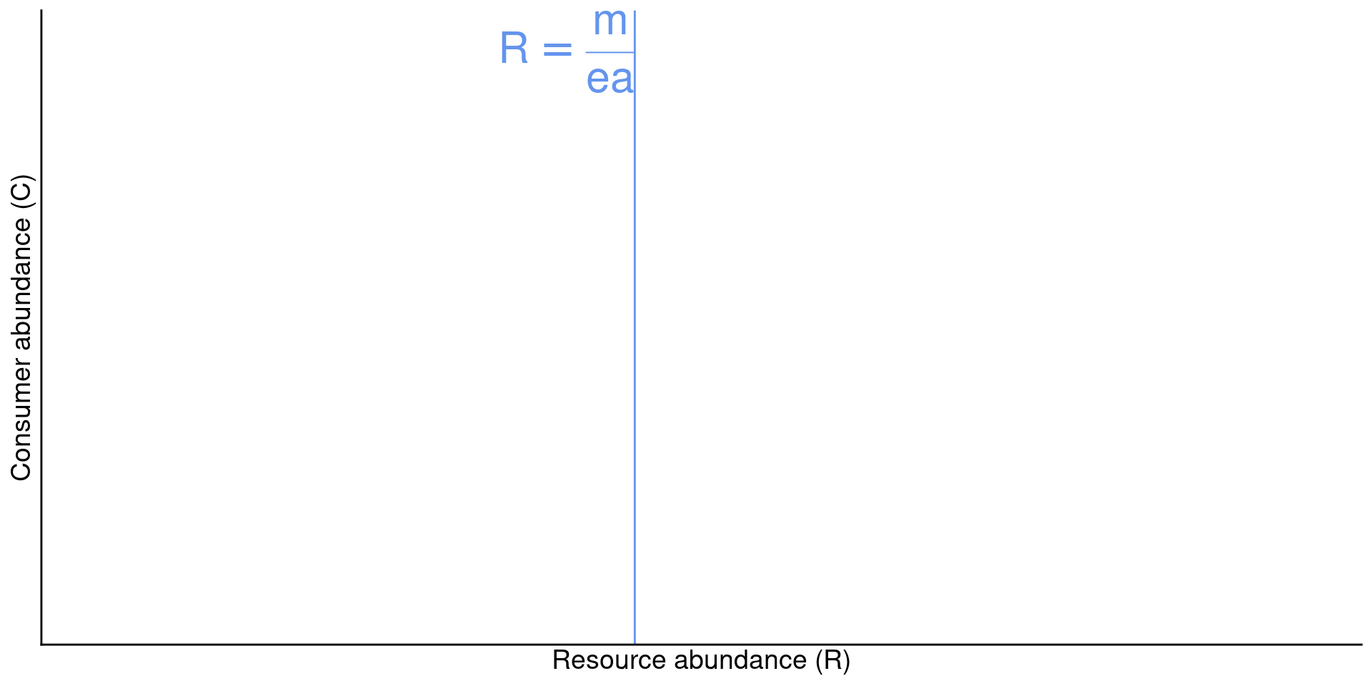
\[R = \frac{m}{ea}\]
Interpration: There is a set abundance of the resource \(R\) that would cause the consumer to reach equilibrium
If the consumer has a high maintenance cost \(m\), this happens at a high value of \(R\)
If the consumer has high attack rate and/or a high conversion efficency, it equlibrates at lower abundances of the resource.
Putting the isoclines together
This suggests that populations should cycle. Do they?
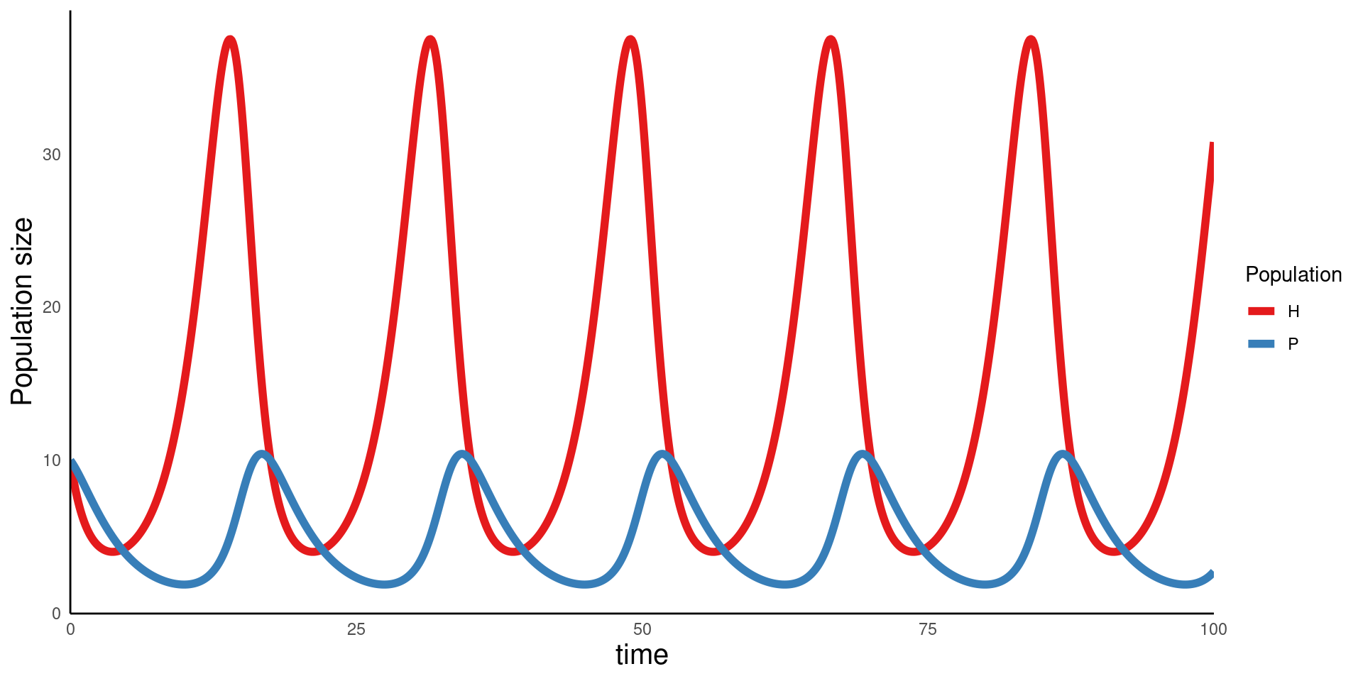
Population cycling in the model
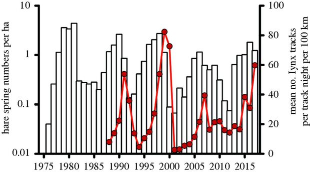
Population cycling in nature
Image from “Population cycles: generalities, exceptions and remaining mysteries”, Meyers 2018 in Proc. Royal Soc. B.
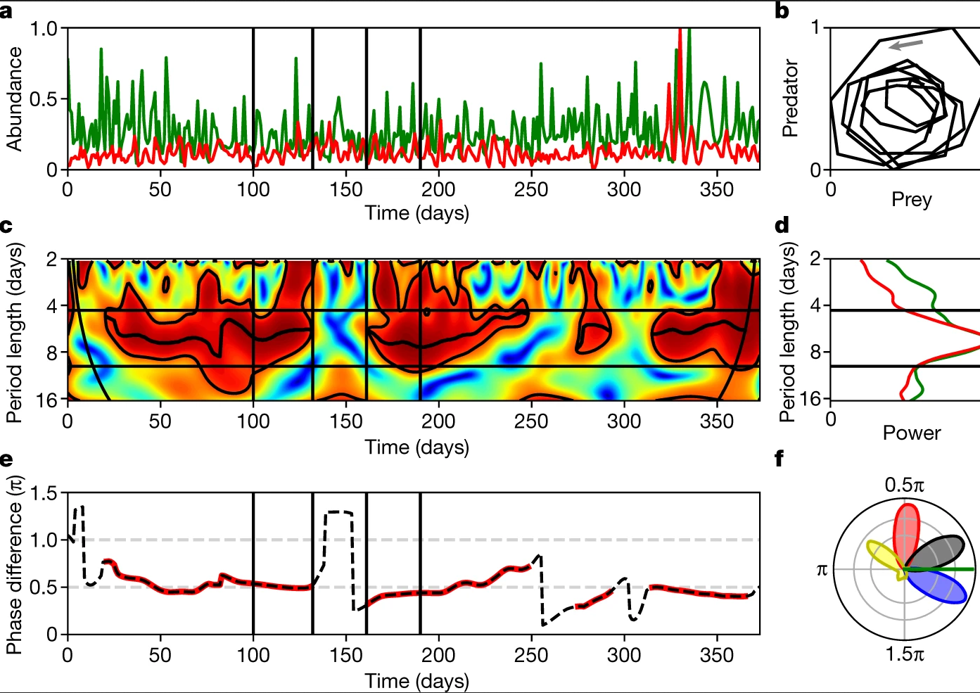
Image from Blasius et al. “Long-term cyclic persistence in an experimental predator–prey system”, 2020, in Nature. These authors were studying a lab population of an aquatic rotifer (consumer) and a grean algae (resource)
Organisms as consumers and resources Day 2
From Monday
Simplified model of consumer–resource dynamics, with a number of assumptions:
Resource species has exponential growth (only limit is from the consumer)
Consumer species is a specialist (only eats the resource species)
Simplified model of consumer–resource dynamics:
\[\frac{dR}{dt} = rR - aRC\]
\[\frac{dC}{dt} = eaRC - mC\]
Equilibrium analysis
Set \(\frac{dR}{dt} = 0\) and \(\frac{dC}{dt} = 0\)
\[\frac{dR}{dt} = rR - aRC\]
\[\frac{dC}{dt} = eaRC - mC\]
Resource equilibrium occurs when \(C = \frac{r}{a}\), Consumer equilibrium occurs when \(R = \frac{m}{ea}\)
Equilibrium analysis
This suggests that consumer and resource populations should be fluctuating
The population abundances do fluctuate in the model dynamics…
… and there’s also evidence that this happens in nature
Image from “Population cycles: generalities, exceptions and remaining mysteries”, Meyers 2018 in Proc. Royal Soc. B.
Image from Blasius et al. “Long-term cyclic persistence in an experimental predator–prey system”, 2020, in Nature. These authors were studying a lab population of an aquatic rotifer (consumer) and a grean algae (resource)
Models as building blocks
The classical model makes some assumptions
Exponential population growth of the resource
Specialist consumer that only eats the focal species we are modeling
But, we now know enough about simple models to see how we can make different pieces fit together
e.g. Consider a pair of resource species (e.g. two grasses that are consumed by a rabbit; two fish species that are consumed by eagles) that also compete with one another
What would a model of their interactions look like?
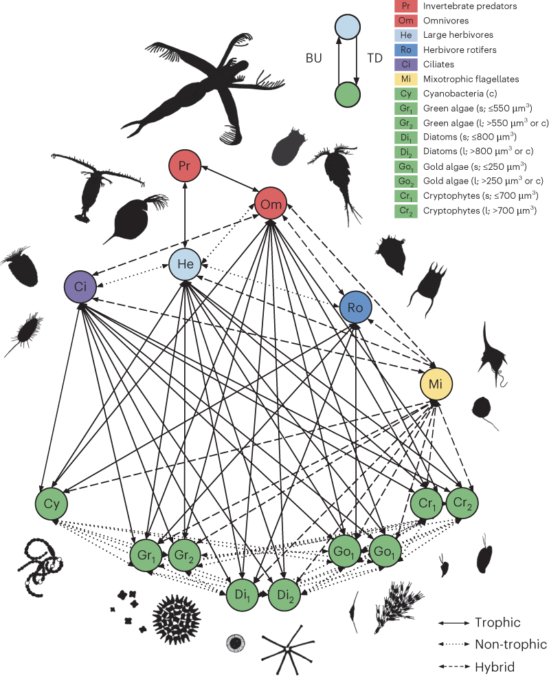
Natural tropic dynamics are often complex
Conceptual diagram of an interaction network in Swiss lakes, from Merz et al 2023 in Nature Climate
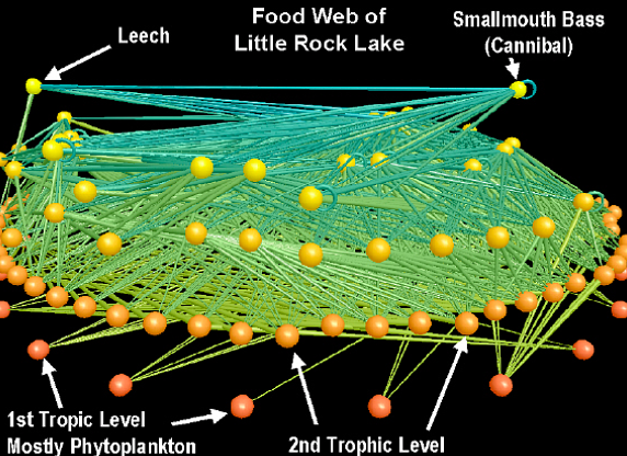
Natural tropic dynamics are often complex
Interaction network of 193 species in Little Rock Lake, Wisconsin; data from Martinez 1991
What are the consequences of perturbing a whole network?
Let’s start by considering a tri-trophic interaction network.
What do you think would happen if the top consumer were to be removed?
What if the middle consumer were to be removed?
What if the resource were to be removed?
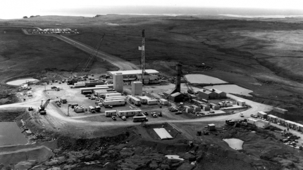
Origins of this idea
Nuclear testing at Amchitka island; see here for more details
The nuclear testing affected otters…
James A. Estes, a University of Arizona doctoral candidate in biology under Atomic Energy Commission contract for an otter study made the estimate of 900 to 1,100 dead otters. (From New York Times, December 1971)
And Jim Estes continued studying these islands, and its otters, through a long career. Estes chronicles his career in the 2016 memoir “Serendipity : An Ecologist’s Quest to Understand Nature”; ebook available through LSU Library
Trophic cascades as important processes structuring ecosystems around the world