flowchart LR
  Susceptible --> Infected --> Recovered
Organisms as resources and consumers
Part 2
Overarching questions in Consumer–resource dynamics
- What allows persistence of consumers and resources in the long term?
- Are there conditions in which consumers “over-consume” and engineer their own demise?
- How does perturbation of the system (e.g. removal of a “top predator”) affect the network as a whole?
Review from Wednesday
- Simple models as “building blocks” for more complicated systems
Consider a system with two species (\(R_1\) and \(R_2\)) that compete with one another for resources, but that are also predated on by the same predator (\(C\)).
Write a model that captures the interactions in this system.
For competing species \(R_1\) and \(R_2\):
\[\frac{dR_1}{dt} = r_1R_1(1-\alpha_{11}R_1 - \alpha_{12}R_2)\] \[\frac{dR_2}{dt} = r_2R_2(1-\alpha_{22}R_2 - \alpha_{21}R_1)\]
Modify these to account for consumer effects:
\[\frac{dR_1}{dt} = r_1R_1(1-\alpha_{11}R_1 - \alpha_{12}R_2)-a_1R_1C\] \[\frac{dR_2}{dt} = r_2R_2(1-\alpha_{22}R_2 - \alpha_{21}R_1)-a_2R_2C\]
The consumer equation also needs to reflect both sources of food:
\[\frac{dC}{dt} = e_1 a_1 R_1 C + e_2 a_2 R_2 C - mC\]
- In the reductionist tradition, we can use these building blocks to logically think through the types of communities that might exist in nature
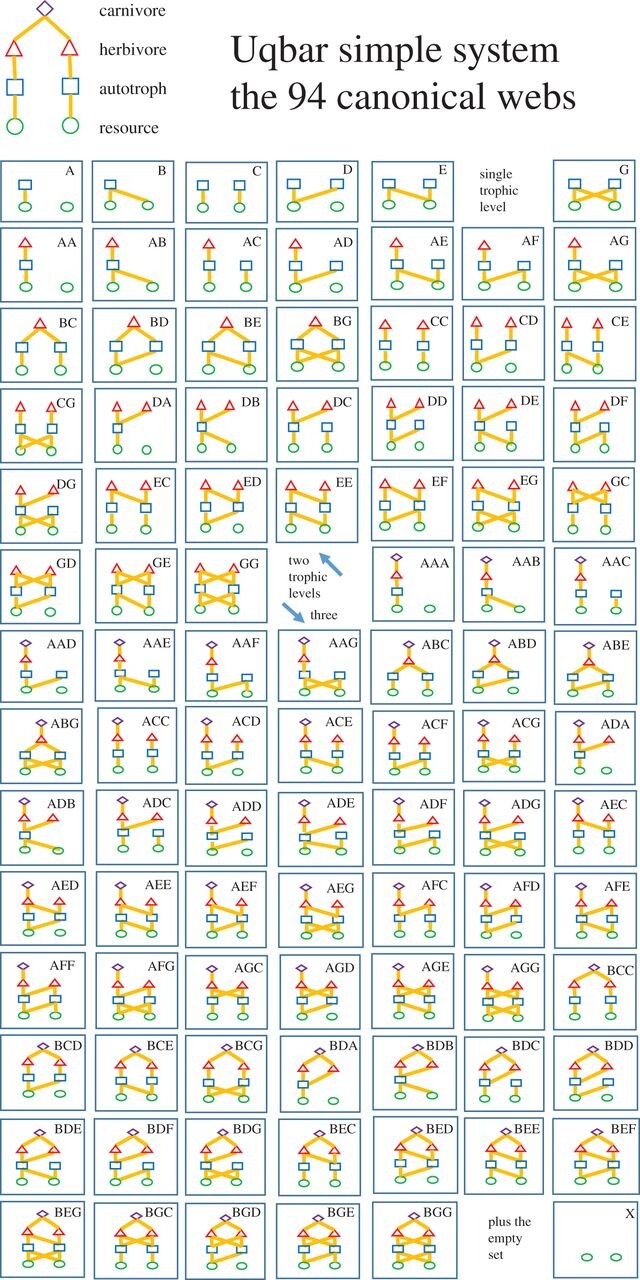
Figure from Bell and Fortier-Dubois 2017, Proc B
Such simplification enables predictions, e.g. what should we expect to happen if one of the herbivores is eliminated?
Of course, there’s some limit to how complicated a system we can reasonably model
- We will begin discussing less reductionist approaches next week.
Three-trophic system
One producer, an herbivore, and a carnivore
e.g. Kelp, sea urchins, and otters
Watch the following two videos if you missed Wednesday
How would we model this?
- Write a simple model of the kelp–urchin–otter system
Assumptions:
- Kelp experiences exponential growth but gets consumed by urchins
- Urchins specialize on kelp as their food source, and are consumer by otters
- Otters primarily eat otters, but they also consume other prey species (e.g. various fish species)
General approach
- Identify the state variables (in our case, \(K\)elp, \(U\)rchin, \(O\)tter)
- Determine what assumptions you are willing to make about the system
- Use our building blocks to start putting together a model
Applying this logic to build a model of infectious disease
Let’s start with some history
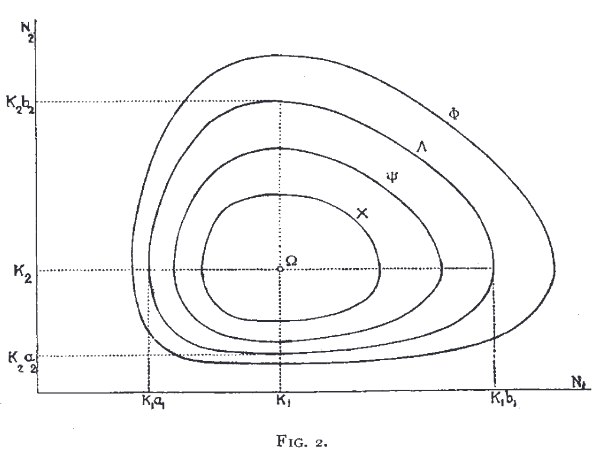
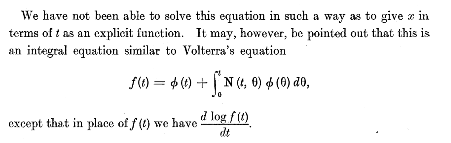
In 1926-27, Volterra and Lotka developed the model of consumer–resource dynamics

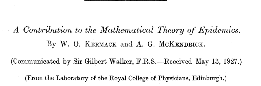
Kermack and McKendrick’s model
Assumptions
- In our focal population, individuals are either \(S\)usceptible to a given disease, are currently \(I\)nfected with the disease, or have recently \(R\)ecovered from the disease.
- (The model is often called the \(SIR\) model for this reason)
- \(S\)usceptible individuals get infected at a rate \(\beta\) when the encounter individuals that are currently \(I\)nfected
- \(I\)nfected individuals recover from infection at a rate \(\gamma\)
- This is equivalent to saying that infected individuals stay infected for \(\frac{1}{\gamma}\) amount of time
- \(R\)ecovered individuals have immunity from the disease for life
- This could make sense for a non-fatal disease that moves through quickly
- E.g. the disease moves quickly enough that we don’t need to think about any births happening in the population
- We can modify the model for diseases that behave differently (e.g. what if recovered individuals lose their immunity over some period of time?) . . .
Assumptions
- In our focal population, individuals are either \(S\)usceptible to a given disease, are currently \(I\)nfected with the disease, or have recently \(R\)ecovered from the disease.
- (The model is often called the \(SIR\) model for this reason)
- \(S\)usceptible individuals get infected at a rate \(\beta\) when the encounter individuals that are currently \(I\)nfected
- \(I\)nfected individuals recover from infection at a rate \(\gamma\)
- This is equivalent to saying that infected individuals stay infected for \(\frac{1}{\gamma}\) amount of time
- \(R\)ecovered individuals have immunity from the disease for life
To model this system we need three equations: \(\frac{dS}{dt}\), \(\frac{dI}{dt}\), \(\frac{dR}{dt}\)
\[\frac{dS}{dt} = -\beta SI\]
\[\frac{dI}{dt} = \beta SI - \gamma I\]
\[\frac{dR}{dt} = \gamma I\]
What do we expect to happen in this system?
\[\frac{dS}{dt} = -\beta SI\]
\[\frac{dI}{dt} = \beta SI - \gamma I\]
\[\frac{dR}{dt} = \gamma I\]
- The number of susceptible individuals is always declining
- Eventually, every individual will get infected, and will eventually recover
- At equilibrium, all individuals will be in the Recovered category
What if the system is more complicated?
- E.g. individuals lose immunity over time
flowchart LR
  Susceptible --> Infected --> Recovered
  Recovered --> Susceptible
- E.g. what if there is a vaccine that allows people to gain immunity without becoming infected?
flowchart LR
  Susceptible --> Infected --> Recovered
  Susceptible --> Vaccinated
- E.g. what if the disease is fatal, such that not all infected individuals recover?
flowchart LR
  Susceptible --> Infected --> Recovered
  Infected --> Dead
Some disease move through populations slowly enough that vital rates (birth and daeth rates) become important
- Are newborns susceptible or immune (innate/maternal immunity)?
Some diseases exist in which there are individuals who are carriers but not infected. These carriers don’t get sick but can get others sick.
Some diseases have an ‘Incubation’ period after infection (i.e. infected individual doesn’t immediately show signs of infection)
Stage/age structure: some diseases cause more effects in older or younger patients – combining matrix model approaches with SIR approach
Next class
- Some lessons from compartment models for understanding disease dynamics
Ecology of infectious diseases
Consider a simple model of disease dynamics (“SIR”)
flowchart LR
  Susceptible --> Infected --> Recovered
- Rate of transmission: \(\beta\)
- Rate of recovery: \(\gamma\)
- Consider a “closed” population: infection is rapid-acting, so births and deaths are not relevant for now.
- For simplicity, define \(S, I, R\) as the proportion of individuals in each compartment
\(S = \frac{\text{total susceptible}}{\text{total number of individuals}}\),
\(I = \frac{\text{total infected}}{\text{total number of individuals}}\)
\(R = \frac{\text{total recovered}}{\text{total number of individuals}}\)
flowchart LR
  Susceptible --> Infected --> Recovered
\[\frac{dS}{dt} = -\beta SI\]
\[\frac{dI}{dt} = \beta SI - \gamma I\]
\[\frac{dR}{dt} = \gamma I\]
Insights from the SIR model
In infectious disease modeling, an important question is:
Under what conditions would a new disease spread through a population?
- Consider a population that has never before encountered a particular disease
- There is no innate immunity, so all individuals are currently in the \(S\)usceptible compartment (\(S = N\))
- One individual gets infected (\(I = 1\), \(S = (N-1)\))
- “Patient zero”
- Will the disease spread, or will it be contained to just Patient Zero?
- In other words: will \(I\) grow or shrink?
- \(\frac{dI}{dt} > 0\)
Insights from the SIR model
To know whether an infection will spread, we need to know whether the following is true:
\[\frac{dI}{dt} = \beta SI - \gamma I \gt 0\]
- If true, infection spreads
- If not true, the infection should disappear over some time
What needs to be true for
\[\frac{dI}{dt} = \beta SI - \gamma I \gt 0\]
\[\beta SI - \gamma I \gt 0\]
\[\beta SI \gt \gamma I\]
\[\beta S \gt \gamma \]
- In this population, most individuals are susceptible (only 1 is infected)
- We defined \(S\) as the proportion of individuals that are susceptible – nearly everyone is!
- So, \(S \approx 1\)
\[\frac{\beta}{\gamma} > 1 ~~~\text{for}~~~ \frac{dI}{dt} > 0\]
\[\frac{\beta}{\gamma} > 1 ~~~\text{for}~~~ \frac{dI}{dt} > 0\]
On the other hand, for the disease to not spread,
\[\frac{\beta}{\gamma} < 1 ~~~\text{for}~~~ \frac{dI}{dt} < 0\]
We give this number a special name:
\[\overbrace{R_0}^{\substack{\text{basic} \\ \text{reproductive} \\ \text{rate}}} = \frac{\beta}{\gamma}\]
- Number of new infections per infector in a population
What controls \(R_0\)
\[R_0 = \frac{\beta}{\gamma}\]
\(R_0 > 1\) implies an infection can spread; \(R_0<1\) implies an infection cannot spread
\(R_0\) can change over time (e.g. because of change virulence of the disease or change in behavior), so we can focus on \(R_{0,t}\) (\(R_0\) at a given time \(t\))
When is \(R_{0, t}\) big?
What can we do to reduce \(R_{0, t}\)?
- Decrease \(\beta\)
- Increase \(\gamma\)
\(R_{0,t}\) is used by public health agencies to monitor trends:
https://www.cdc.gov/cfa-modeling-and-forecasting/rt-estimates/index.html
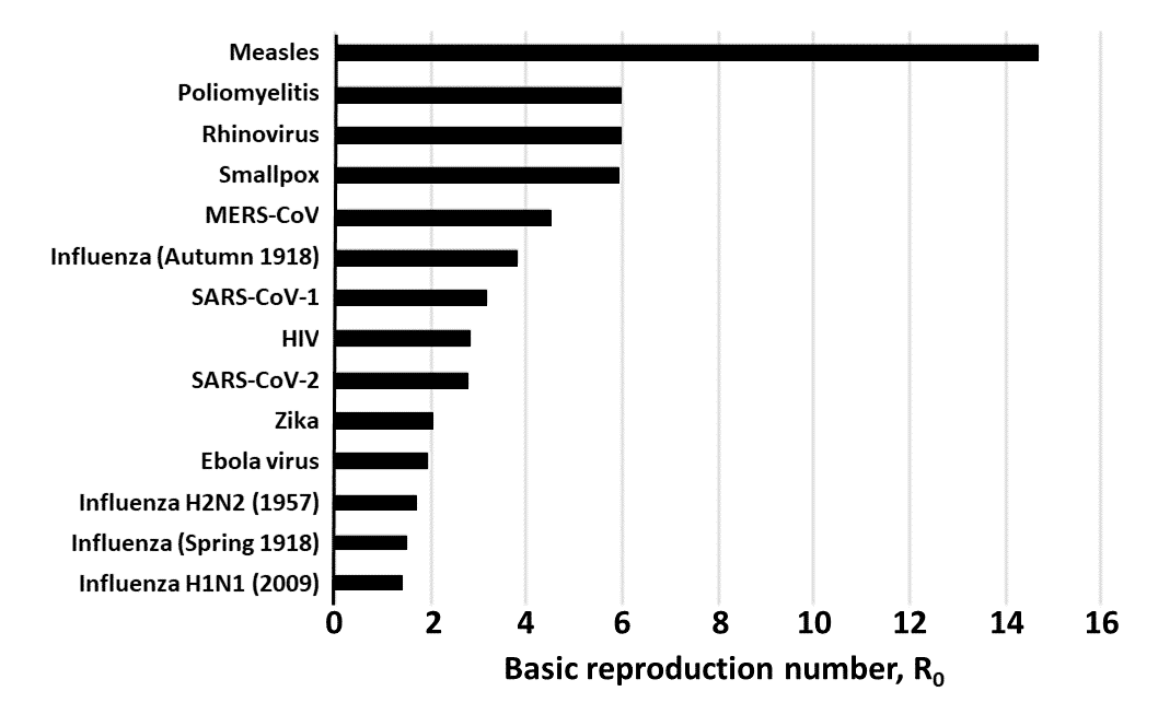
\(R_0\) for important infections, from the Center for Evidence Based Medicine, Oxford Univ.
Infectious disease ecology wrapup
\[\frac{dS}{dt} = -\beta SI\]
\[\frac{dI}{dt} = \beta SI - \gamma I\]
\[\frac{dR}{dt} = \gamma I\]
- If a new disease emerges, will it spread or not?
\[\frac{dI}{dt} = \beta SI - \gamma I\]
- When is this above zero?
\[\beta SI > \gamma I\]
\[\beta S > \gamma\]
- When a disease first emerges, almost everyone will be susceptible to it: \(S \approx 1\)
\(\beta > \gamma\), aka \(\frac{\beta}{\gamma} > 1\)
\[\frac{\beta}{\gamma} > 1\]
We give the ratio \(\frac{\beta}{\gamma}\) a special name: \(R_0\) (“R-naught”) or basic reproductive rate of the disease
If \(R_0>1\), the disease is predicted to spread after it first enters the system; otherwise, it cannot spread.
Recall that the assumption behind \(R_0\)’s equation is that we are thinking about the disease immediately after it enters the population, so \(S \approx 1\)
- But as a disease circulates through a population, this will change – many individuals will be infected and (hopefully) recovered
So in real life, disease ecologists track \(R_t\), or disease reproductive rate at a given time.
\[R_0 = \frac{\beta}{\gamma}\]
Reducing \(R_0\) requires either reducing \(\beta\) or increasing \(\gamma\)
\(\beta\) is the transmission probability if an interaction does happen – can be hard to modify
\(\gamma\) is the recovery rate of infected individuals – can be hard to lower for brand new infections
Over time, these numbers can change, e.g. due to evolution of the infectious disease itself or due to better recovery
But at the time of disease introduction, these can be hard
Reducing disease spread without altering \(R_0\)
- Reducing \(R_0\) requires reducing \(\beta\), but if we can’t, the next best thing is to have fewer interactions between Susceptible and Infectious individuals:
\[\frac{dS}{dt} = -\beta SI\]
\[\frac{dI}{dt} = \beta SI - \gamma I\]
\[\frac{dR}{dt} = \gamma I\]
Fewer interactions requires measures like quarntining, or moving individuals out of the \(S\)uscptible category – which is possible through vaccination.
Other resources for learning about applications of SIR models:
https://media.hhmi.org/biointeractive/click/modeling-disease-spread/advanced-simulate.html
Modeling Epidemics With Compartmental Models, overview by JAMA (Journal of the American Medical Association)
Video series by US CDC: https://www.youtube.com/watch?v=1QLgXzyXOH0