Week 10
Quantifying biodiversity
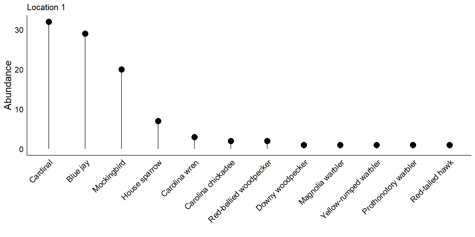
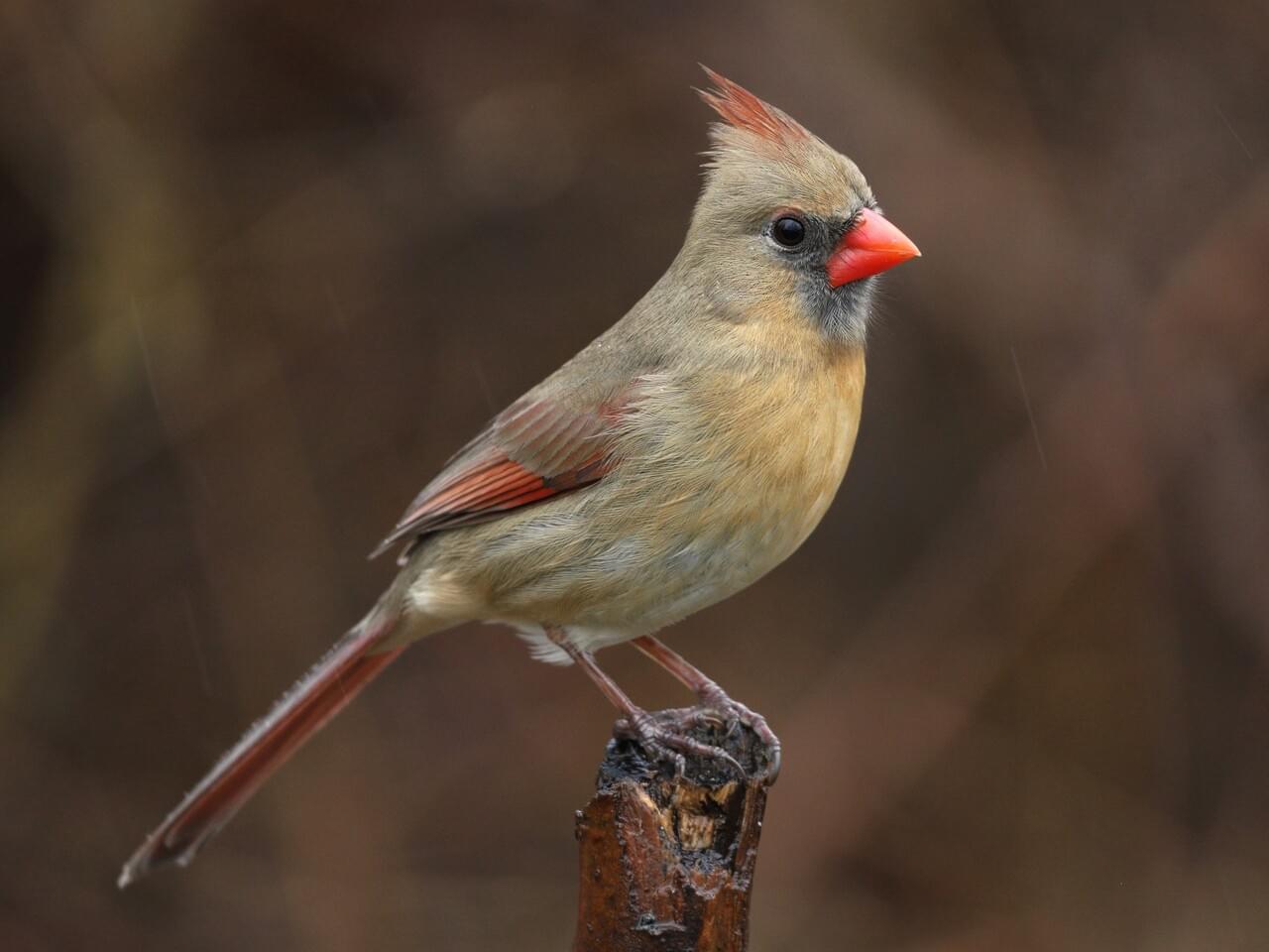
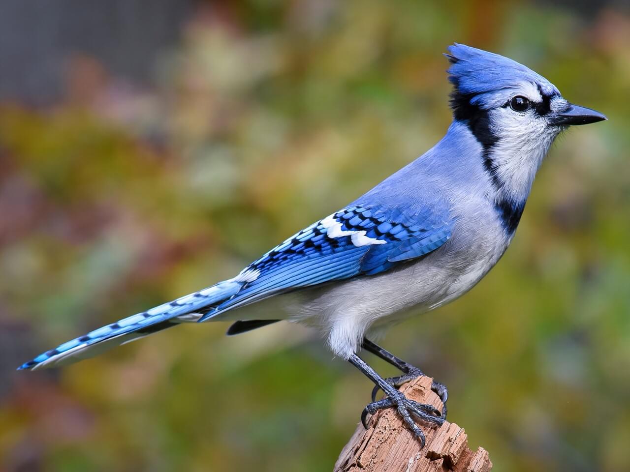
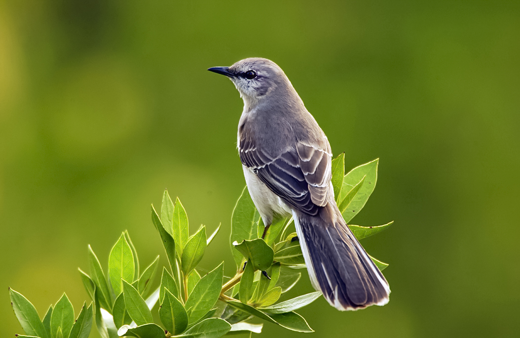
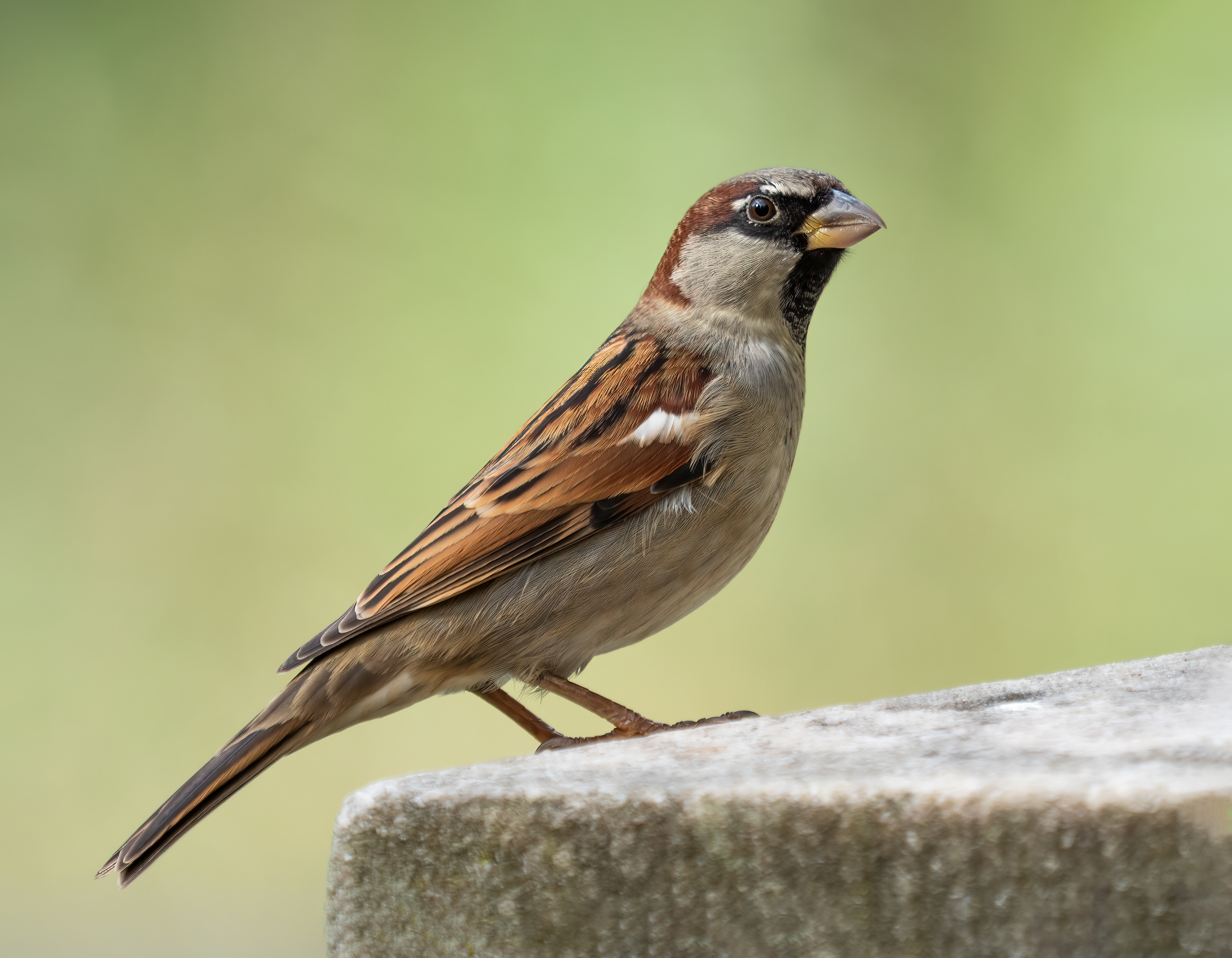
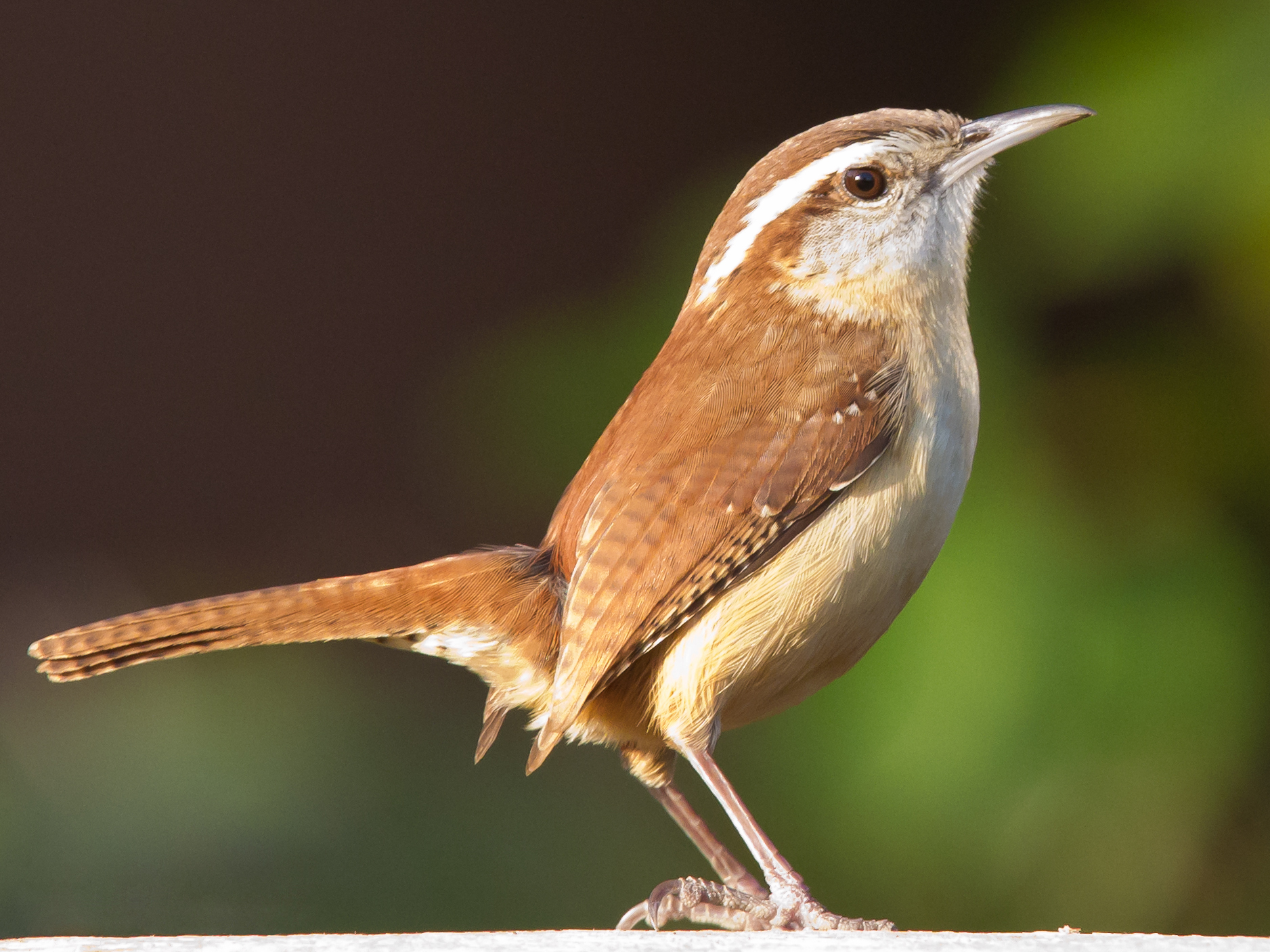
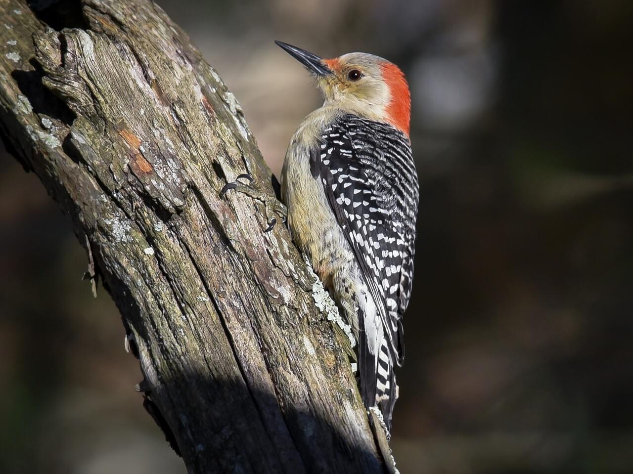
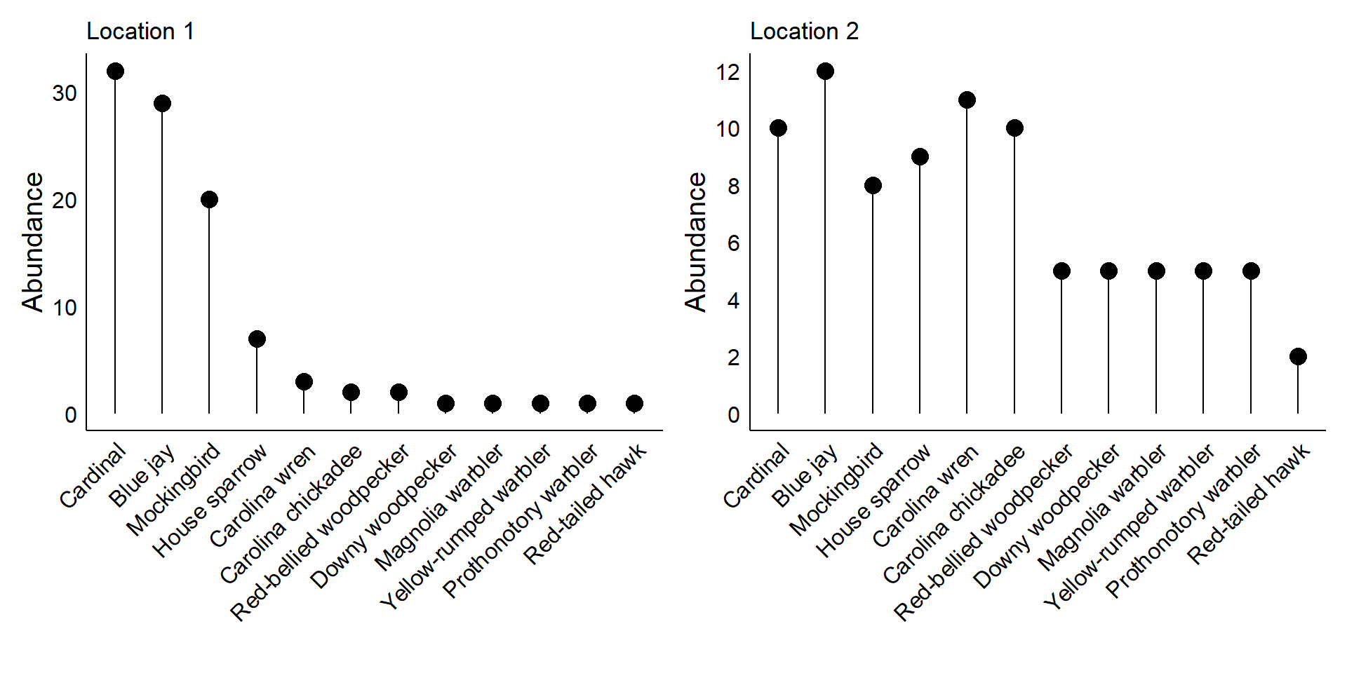
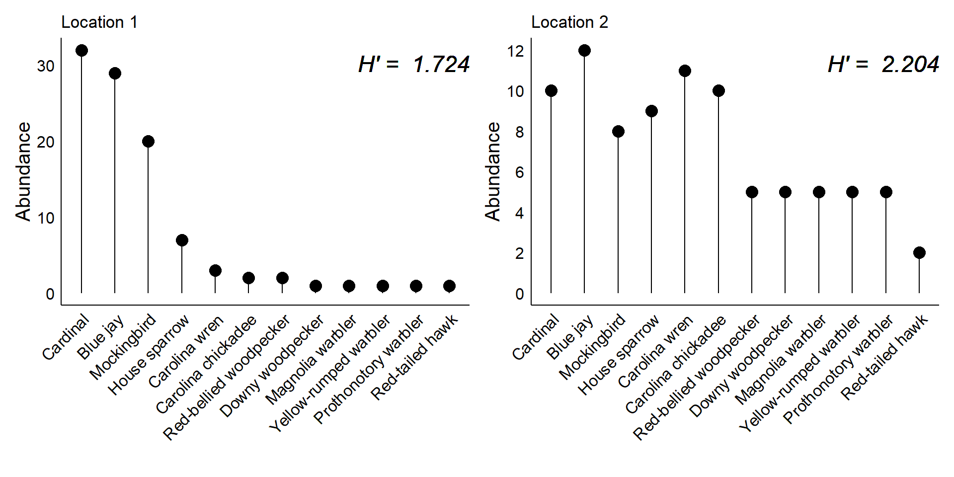
Some common birds of Baton Rouge


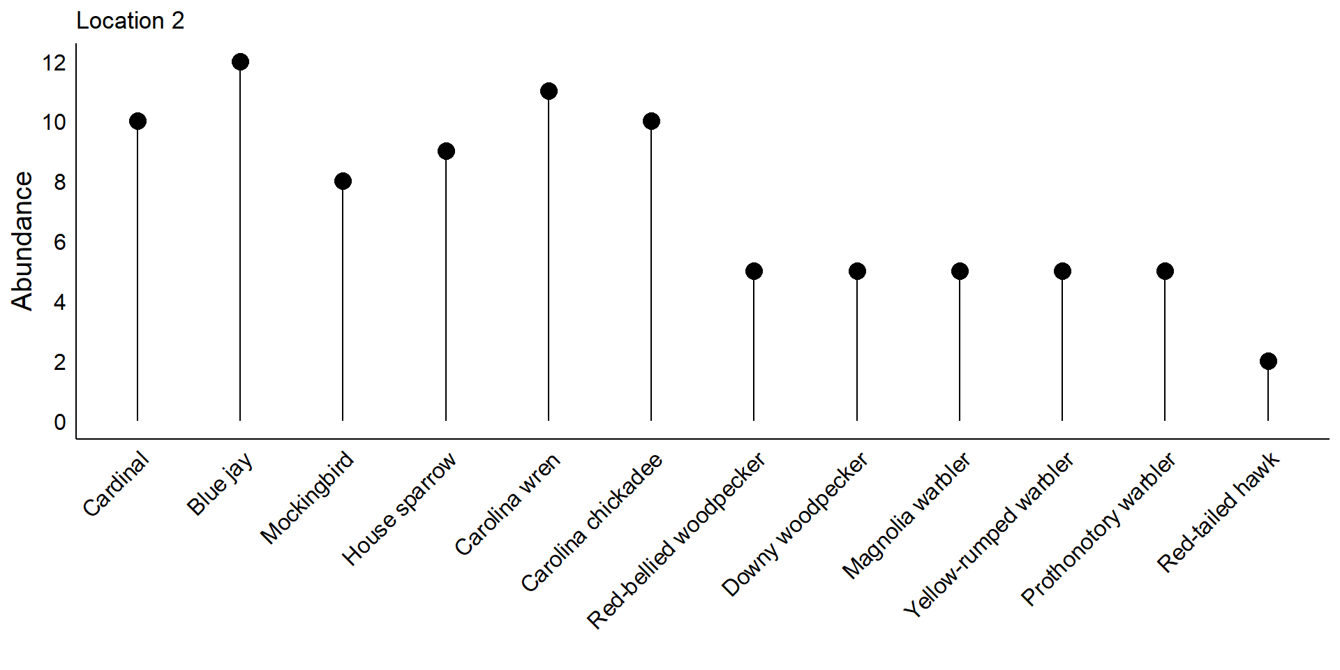
In second location, individuals from each species are fairly common:

Small group discussion:
What is the biodiversity in each location?
If you go to Location 1 vs. Location 2 and spend 10 minutes in each, do you think you would see an equal number of species?
Community 1


Community 2
- Communities can have different amount of “Phylogenetic history” represented in their species list
Accounting for variation in abundance

- If I were randomly finding birds in Location 1 and had to guess which species I would find next, which should I guess?
Shannon diversity index

- How about in Location 2?
Shannon diversity index

- Location 1 is more “predictable”
- Higher degree of “surprise” in Location 2
- This is also called “Information entropy”
- Commonly used across science, e.g. in computers, to optimize information storage and transfer
Shannon diversity index
A quantitative measure of biodiversity and community “evenness”
\[\overbrace{H'}^{\substack{\text{Shannon}\\{\text{index}}}} = -\sum_{i = 1}^{n} \overbrace{p_i}^{\substack{\text{proportional}\\ \text{abundance}}}*\overbrace{\text{ ln}(p_i)}^{\log\big(\substack{\text{proportional}\\ \text{abundance}}\big)}\]

University Lakes bird biodiversity
University Lakes bird biodiversity

Shannon diversity: a measure of “surprise”
The geographic scales of biodiversity

pop quiz: how many species of native plants are in Louisiana?
“Did you know that Louisiana has about 2,500 native plants?”
But, not all plants are everywhere!


Biodiversity patterns in action
In the following communities, each species is represented by a different letter.
Let’s calculate \(\alpha\), \(\beta\), and \(\gamma\) diversity.
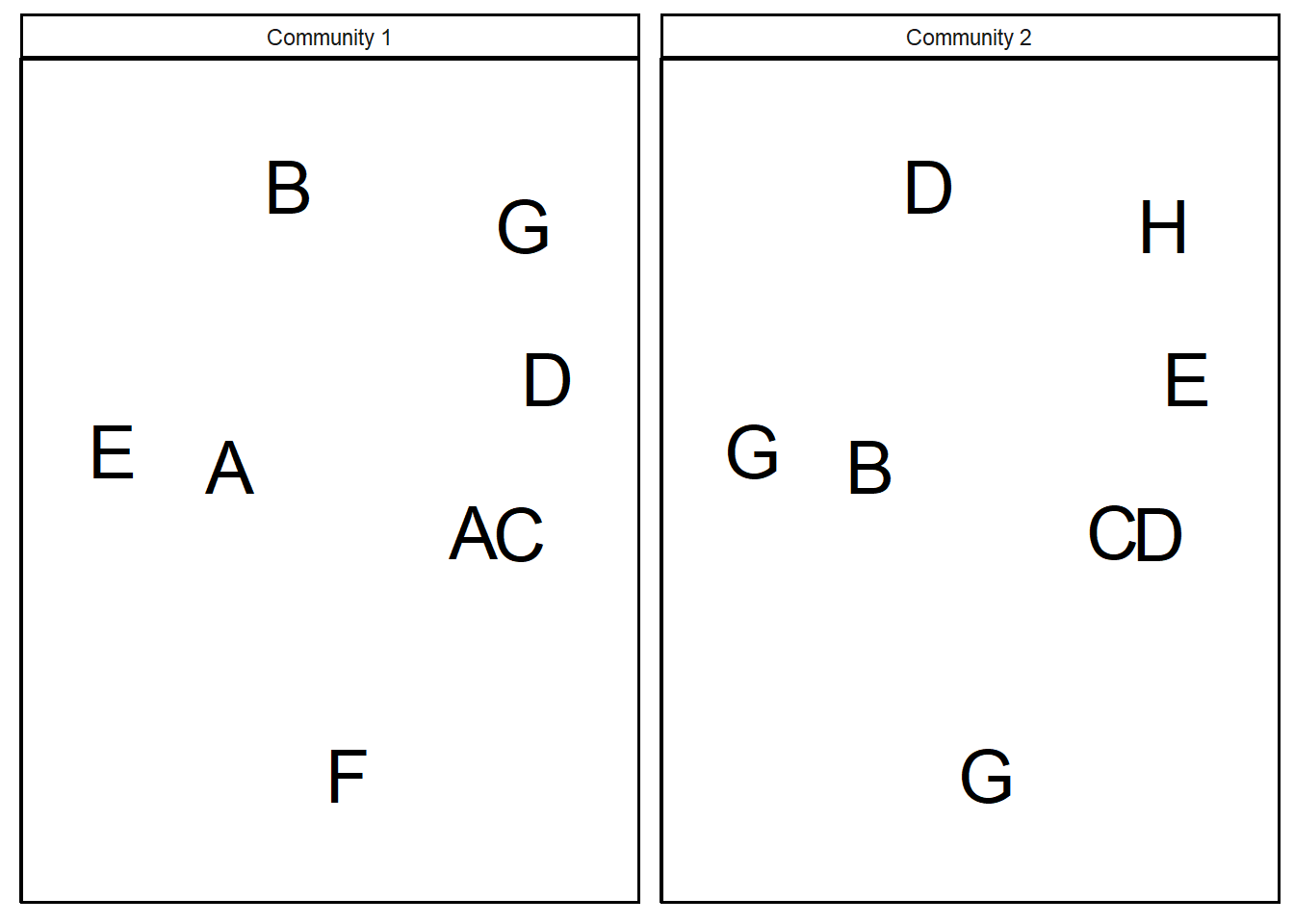
\(\alpha_{\text{community }1} = 7 \text{ species}\)
\(\alpha_{\text{community }2} = 6 \text{ species}\)
\(\gamma = 8 \text{ species}\) (A,B,C,D,E,F,G,H)
\(\beta\) is the number of species unique to one community
- Species \(A\) and \(F\) only in Community 1
- Species \(H\) only in Community 2
- \(\beta = 3\) unique species
Your turn: calculate \(\alpha\), \(\beta\), and \(\gamma\) diversity for the following

- \(\beta\) diversity is an important and complicated concept

Why bother?!
Quantifying patterns of biodiversity is essential for getting a good grasp on managing and protecting biodiversity
More on this in the next two weeks.